

Compositional symmetry between Earth’s crustal building blocks
Affiliations | Corresponding Author | Cite as

- Share this article


-
Article views:11,989Cumulative count of HTML views and PDF downloads.
- Download Citation
- Rights & Permissions

Abstract
Figures and Tables
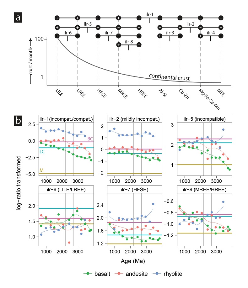
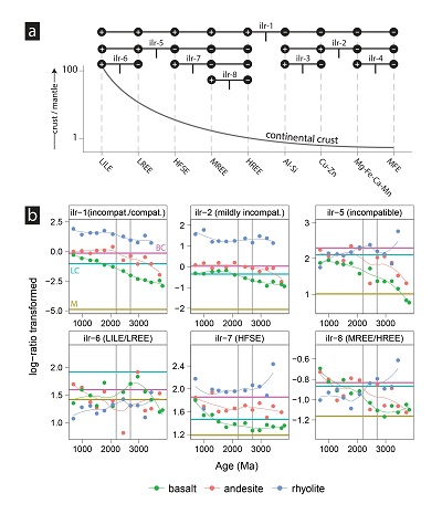 Figure 1 (a) Schematic spider diagram plotting the composition of the continental crust, normalised to primitive mantle, in relation to isometric-log-ratios (ilr). Numerators and denominators for each ilr-balance are denoted by plus and minus signs, respectively. Each ilr represents a ratio between elements with contrasting compatibility during mantle melting. (b) Geochemical evolution of basalt, andesite, and rhyolite magmas based on ilr. Aggregated log-ratio means and loess-curves are colour coded to rock type. Vertical, grey lines represent the Archean-Palaeoproterozoic boundary (2.7–2.2 Ga; Condie and O’Neill, 2010). Basaltic and andesitic rocks have become incompatible element-rich through time resulting in a negatively sloping ilr-1. Rhyolitic rocks have also become incompatible element-rich (ilr-1), but to a lesser extent and, for some log-ratios (ilr-5–8), yield contrasting trends (positive slopes) that may track the evolving composition of their basaltic to andesitic source. Horizontal lines represent mantle (M; Palme and O’Neill, 2014) and crustal compositions (LW = lower crust; BC = bulk continental crust; Rudnick and Gao, 2003) and are shown for reference. Abbreviations: LILE = large ion lithophile (K, Na, Ba, Sr, Rb, Pb, Cs), LREE = light rare earth element (La, Ce, Pr, Nd); HFSE = high field strength elements (Ti, P, Zr, Hf, Nb, Ta, U, Th); MREE = middle rare earth element (Sm, Eu, Gd); HREE = heavy rare earth element (Tb, Dy, Ho, Er, Yb, Lu, Y); MFE = mantle forming elements (Cr, Ni, Co, Ga, Sc, V). | 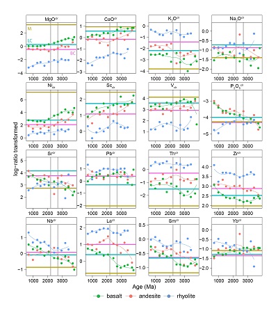 Figure 2 Geochemical evolution of basalt, andesite and rhyolite on an element-by-element basis following a centred log-ratio (clr) approach (Aitchison, 1986). Vertical, grey lines represent the Archean-Palaeoproterozoic boundary (2.7–2.2 Ga; Condie and O’Neill, 2010). Horizontal lines represent mantle (M; Palme and O’Neill, 2014) and crustal compositions (LW = lower crust; BC = bulk continental crust; Rudnick and Gao, 2003) and are shown for reference. This log-ratio transformation preserves a one-to-one relationship with the original variables, but adding or removing variables changes the absolute value of each clr (see Supplementary Information). Isometric log-ratios (Fig. 1) are not restricted by this constraint and represent the preferred approach for compositional data analysis (Egozcue et al., 2003). | 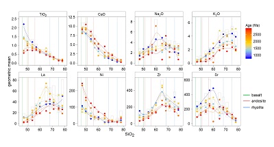 Figure 3 Harker diagrams based on the geometric mean of raw SiO2 concentrations. Individual curves are colour coded to age and represent globally averaged, liquid lines of descent for each time slice. Vertical lines represent the inter-quartile range for each rock type. Vertical grey boxes represent the inter-quartile range for each element at any given SiO2 bucket. Overall, ancient crystal fractionation for compatible elements are displaced to lower values at any given SiO2 bucket, consistent with the partial mantle-melt trend based on log-ratios. |
| Figure 1 | Figure 2 | Figure 3 |
Supplementary Figures and Tables
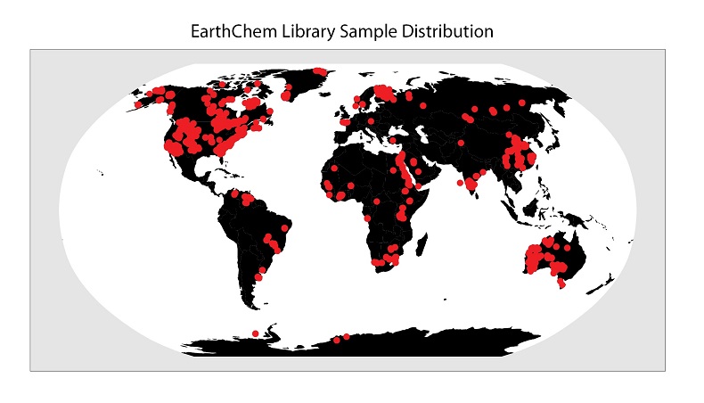
 Figure S-1 Geographic distribution of Precambrian EarthChem Library samples included within the present study. |  Figure S-2 (a) Complete cases (black) versus imputed (red) kernel density distributions for TiO2. (b-c) Overall, the imputed values are realistic and do not affect the secular trends that are the focus herein. Error-bars are reported as 2 × standard error of the mean. |  Figure S-3 Boxplot distributions for complete-cases (black) versus the imputed dataset (dots represent outliers). Imputed values do not significantly affect the central tendency for elements that possess between 10 and 50 % missing values (left to right). | 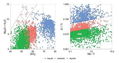 Figure S-4 TAS (left) and Pearce (right) rock classification diagrams colour coded to rock type. Only the first 100 (out of 10,000) re-sampled datasets are shown for clarity. Rock names: 1 = picro-basalt; 2 = basalt; 3 = basaltic andesite; 4 = andesite; 5 = dacite; 6 = rhyolite; 7 = basanite; 8 = trachy-basalt; 9 = basaltic trachy-andesite; 10 = trachyte; 12 = phonotephrite; 13 = tephriphonolite; 14 = phonolite; 15 = foidite. |
| Figure S-1 | Figure S-2 | Figure S-3 | Figure S-4 |
 Figure S-5 TAS (left) and Pearce (right) rock classification diagrams colour coded to age. Only the first 100 (out of 10,000) re-sampled datasets are shown for clarity. The tendency for modern rock types to be alkali element-rich is clear even within this simple data projection. Rock names: 1 = picro-basalt; 2 = basalt; 3 = basaltic andesite; 4 = andesite; 5 = dacite; 6 = rhyolite; 7 = basanite; 8 = trachy-basalt; 9 = basaltic trachy-andesite; 10 = trachyte; 12 = phonotephrite; 13 = tephriphonolite; 14 = phonolite; 15 = foidite. | 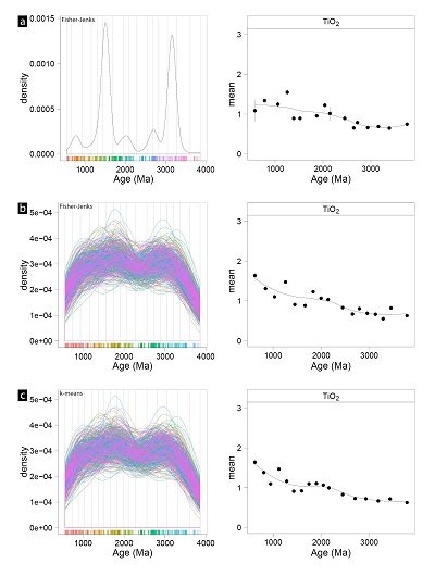 Figure S-6 (a) Original data distribution and secular TiO2 trend fitted with loess. Data clustering is due to the uneven distribution of the igneous rock record and false age-peaks related to poorly-defined ages within the EarthChem library. The impact of this punctuated igneous rock record was minimised by weighted bootstrap re-sampling (weighted inversely to age density; see text for discussion). Vertical lines are age buckets defined by the Fisher-Jenks method. Rug plots are colour coded to age bucket. (b–c) Kernel density distributions for the first 1,000 re-sampled iterations (out of 10,000; density curves are colour coded to iteration number) and secular TiO2 trends fitted with loess. Vertical lines are age buckets defined by the Fisher-Jenks and K-means methods, respectively. Rug plots colour coded to age bucket. Overall, re-sampled data for even this relatively small-number of iterations closely approximates the trend defined by the original dataset. |  Figure S-7 Robust principal component analysis (Templ et al., 2011) colour coded to rock type (left) and age (right) using the original variables. Only the first 1,000 (out of 10,000) re-sampled datasets are shown for clarity. | 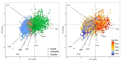 Figure S-8 Robust principal component analysis (Templ et al., 2011) colour coded to rock type (left) and age (right) using element groups. The similarities between this projection and principal component analysis using the original elements (Fig. S-7) suggests that reducing the number of variables does not impact the results. Only the first 1,000 (out of 10,000) re-sampled datasets are shown for clarity. | 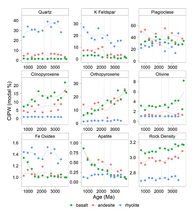 Figure S-9 Normative mineralogy (modal %) based on CIPW calculations using raw major element concentrations in R (Guzman, 2015). Vertical, grey lines represent the Archean-Palaeoproterozoic boundary (2.7–2.2 Ga; Condie and O’Neill, 2010). Extensive partial melting during the Archean exhausted clinopyroxene and fused more refractory minerals such as orthopyroxene and olivine. |
| Figure S-5 | Figure S-6 | Figure S-7 | Figure S-8 | Figure S-9 |
top
Introduction
Igneous rocks are the main building blocks of the continental crust and represent a long-lived and accessible record of Earth’s dynamic geochemical landscape. New continental crust, generated today at convergent and intra-plate settings, is predominately basaltic and thus contrasts with the andesitic composition of the bulk continental crust (Rudnick, 1995
Rudnick, R. (1995) Making continental crust. Nature 378, 571–577.
; Taylor and McLennan, 1995Taylor, S., McLennan, S. (1995) The geochemical evolution of the continental crust. Reviews of Geophysics and Space Physics 33, 241–265.
). This apparent disconnect points to a two-stage, igneous-driven process whereby relatively primitive basaltic magmas are extracted from the mantle and are further differentiated, by re-melting, fractional crystallisation and/or mixing to produce the wide range of igneous rock compositions that are exposed at surface (Hawkesworth and Kemp, 2006Hawkesworth, C., Kemp, A. (2006) Evolution of the continental crust. Nature 443, 811–817, doi: 10.1038/nature05191.
). The compositional symmetry between the evolved continental crust and the relatively depleted mantle is well documented and helps to define our unique place in the solar system (Allègre, 1997Allègre, C. (1997) Limitation on the mass exchange between the upper and lower mantle: the evolving convection regime of the Earth. Earth and Planetary Science Letters 150, 1–6.
; Taylor and McLennan, 2009Taylor, S., McLennan, S. (2009) Planetary Crusts. Cambridge University Press, Cambridge, 404 pp.
).Despite isotopic evidence that suggests the Archean depleted mantle source (at least by 3.8 Ga) was likely similar to today (Vervoort and Blichert-Toft, 1999
Vervoort, J.D., Blichert-Toft, J. (1999) Evolution of the depleted mantle: Hf isotope evidence from juvenile rocks through time. Geochimica et Cosmochimica Acta 63, 533–556, doi: 10.1016/S0016-7037(98)00274-9.
), the processes that shaped the composition of the continental crust in the geologic past are less understood (Bédard et al., 2013Bédard, J.H., Harris, L.B., Thurston, P.C. (2013) The hunting of the snArc. Precambrian Research 229, 20–48.
). Andesitic rocks are central to this debate because they represent the signature rock type at many young arcs and their occurrence in the Precambrian rock record is a key piece of evidence for tracing modern tectonic processes back into the geologic past. Whether these ancient intermediate rock compositions represent primary mantle melts, mixing between differentiated basaltic and rhyolitic melts and/or are crystal fractionation products of basaltic magmas, however, remains controversial (Reubi and Blundy, 2009Reubi, O., Blundy, J. (2009) A dearth of intermediate melts at subduction zone volcanoes and the petrogenesis of arc andesites. Nature 461, 1269–1273, doi: 10.1038/nature08510.
; Lee and Bachmann, 2014Lee, C.-T.A., Bachmann, O. (2014) How important is the role of crystal fractionation in making intermediate magmas? Insights from Zr and P systematics. Earth and Planetary Science Letters 393, 266–274, doi: 10.1016/j.epsl.2014.02.044.
).Herein the shifting compositional relationships between the three main igneous rock types (i.e. basalt, andesite, and rhyolite) map the major geochemical changes that have shaped the continental crust through Earth’s history. The focus is on estimating the geochemical centre, or central tendency, for each element and rock type through time (Aitchison, 1986
Aitchison, J. (1986) The statistical analysis of compositional data. Chapman & Hall, Ltd. London, UK, 416 pp.
; Egozcue et al., 2003Egozcue, J., Pawlowsky Glahn, V., Mateu-Figueras, G., Barceló Vidal, C. (2003) Isometric logratio for compositional data analysis. Mathematical Geosciences 35, 279–300, doi: 10.1023/A:1023818214614.
). This approach is thus distinct from, but complementary to, most previous studies on smaller, well-characterised sample sets that tend to emphasise geochemically anomalous sample sub-sets and/or focus on more specific rock sub-types (e.g., calc-alkaline versus tholeiitic basalts).top
Compositional Data Analysis
Geochemical data, like other forms of compositional data, sum to constant (i.e. closed data) and convey only relative information (Aitchison, 1986
Aitchison, J. (1986) The statistical analysis of compositional data. Chapman & Hall, Ltd. London, UK, 416 pp.
). Log-ratios have emerged as one of the preferred approaches for treating such compositional datasets (Egozcue et al., 2003Egozcue, J., Pawlowsky Glahn, V., Mateu-Figueras, G., Barceló Vidal, C. (2003) Isometric logratio for compositional data analysis. Mathematical Geosciences 35, 279–300, doi: 10.1023/A:1023818214614.
), however, these alternative data treatments can be difficult to interpret in the conventional way, which has limited the application of log-ratio analysis to petrologic problems. Herein log-ratios are based on the order of element compatibility during mantle melting to facilitate their petrologic interpretation. Elements were also grouped to further simplify log-ratio analysis and to summarise temporal trends. This particular form of log-ratio analysis is thus comparable to the usual approach of linking petrogenetic processes to patterns on multi-element diagrams, or so-called spider plots. Slope changes on these classic diagrams, which can be further reduced to ratios (or log-ratios in this case) between elements of contrasting compatibility (incompatible versus compatible elements), reflect igneous differentiation processes such as the degree of partial melting and/or fractional crystallisation (Pearce, 2008Pearce, J.A. (2008) Geochemical fingerprinting of oceanic basalts with applications to ophiolite classification and the search for Archean oceanic crust. Lithos 100, 14–48, doi: 10.1016/j.lithos.2007.06.016.
). However, in comparison to interpretations based on raw element concentrations, log-ratios reflect the actual relationships between element groups rather than the spurious effects related to the closed nature of compositional data (Egozcue et al., 2003Egozcue, J., Pawlowsky Glahn, V., Mateu-Figueras, G., Barceló Vidal, C. (2003) Isometric logratio for compositional data analysis. Mathematical Geosciences 35, 279–300, doi: 10.1023/A:1023818214614.
).top
Data Processing
The full methodological approach is described in the Supplementary Information. Data processing and figures can also be reproduced using the free, open source R software environment (R Core Team, 2015
R Core Team (2015) R: A language and environment for statistical computing. R Foundation for Statistical Computing, Vienna, Austria. URL https://www.R-project.org/.
) and code available from the corresponding author. Geochemical data and age data were compiled from the EarthChem library (Fig. S-1). This global geochemical database contains a relatively large number of missing values for some elements. Most previous studies exclude these missing values and consider only the so-called complete cases; however, the consequences of this default option are rarely, if ever, discussed. Log-ratio analysis requires complete datasets and thus, in this case, missing values for elements with minor to moderate degrees of missingness (typically 10–30 % missing) were replaced using column-wise multivariate imputation by chained equations (van Buuren and Groothuis-Oudshoorn, 2011van Buuren, S., Groothuis-Oudshoorn, K. (2011) mice: Multivariate Imputation by Chained Equations in R. Journal of Statistical Software 45, 1-67.
). The impact of the selected imputation method is evaluated in the Supplementary Methods (Figs. S-2 and S-3).Precambrian samples (≥541 Ma; n = 66,739) were then discretised into basaltic, andesitic and rhyolitic compositions based on the Total Alkali Silica (Le Bas et al., 1986
Le Bas, M., Le Maitre, R., Steckeisen, A., Zanettin, B. (1986) The construction of the total alkali–silica chemical classification of volcanic rocks. Journal of Petroleum Science and Engineering 27, 745–750.
) and Pearce (Pearce, 1996Pearce, J. (1996) A users guide to basalt discrimination diagrams. In: Pearce, J., Wyman, D. (Eds.) Geological Association of Canada, Short Course Notes. Geological Association of Canada, 79–113.
) classification diagrams (Figs. S-4 and S-5). This classification approach uses mobile- and least-mobile elements to reject metasomatised samples, a particularly important step for Precambrian metamorphosed igneous rocks. The remaining igneous samples (n = 18,246) were then split into age groups based on a K-means clustering approach. Weighted bootstrap re-sampling of the data (weighted inversely to age) was used to minimise the effect of unevenly distributed crystallisation ages (Fig. S-6), which are inherent to the punctuated, igneous rock record (Keller and Schoene, 2012Keller, C.B., Schoene, B. (2012) Statistical geochemistry reveals disruption in secular lithospheric evolution about 2.5 Gyr ago. Nature 485, 490–493, doi: 10.1038/nature11024.
). Log-ratios were then calculated from the re-sampled dataset and are presented in Figures 1 and 2.top
Results and Discussion
Isometric log-ratios (ilr-1–8) represent the preferred approach for compositional datasets (Egozcue et al., 2003
Egozcue, J., Pawlowsky Glahn, V., Mateu-Figueras, G., Barceló Vidal, C. (2003) Isometric logratio for compositional data analysis. Mathematical Geosciences 35, 279–300, doi: 10.1023/A:1023818214614.
) and, as defined herein, divide the classic spider diagram into a series of non-overlapping segments (Fig. 1). The first log-ratio (ilr-1) represents the overall proportion of incompatible versus compatible elements (Fig. 1a), whereas the remaining ilrs split the mildly incompatible to compatible (ilr-2–4) and incompatible (ilr-5–8) element portions of the spider diagram into successively smaller segments (Fig. 1a). These smaller segments reflect key petrogenetic indicators such as large ion lithophile element (LILE)- and high field strength element (HFSE)-enrichment (ilr-6 and ilr-7, respectively), and can also be constructed to reproduce commonly used ratios, such as Sm/Yb, which monitor the influence of key mineral phases (e.g., garnet) during melting (ilr-8; Pearce, 2008Pearce, J.A. (2008) Geochemical fingerprinting of oceanic basalts with applications to ophiolite classification and the search for Archean oceanic crust. Lithos 100, 14–48, doi: 10.1016/j.lithos.2007.06.016.
).Basalt and andesite yield negative sloping log-ratios (ilr-1; Fig. 1b), suggesting that these rock types have become increasingly incompatible-element-rich and compatible-element-poor since the Archean. Temporal trends between basaltic and rhyolitic rock types are broadly parallel and yield steadily increasing incompatible versus compatible element log-ratios (ilr-1–8) despite grouping disparate basaltic and andesitic rock sub-types (Fig. 1). On a conventional spider diagram, systematic incompatible element enrichment would correspond to steepening multi-element profiles through time (Fig. 1a). This well-documented pattern is consistent with extensive partial mantle-melting in the geologic past and was possibly driven by hotter, Archean mantle temperatures (Herzberg et al., 2010
Herzberg, C., Condie, K., Korenaga, J. (2010) Thermal history of the Earth and its petrological expression. Earth and Planetary Science Letters 292, 79–88, doi: 10.1016/j.epsl.2010.01.022.
; Keller and Schoene, 2012Keller, C.B., Schoene, B. (2012) Statistical geochemistry reveals disruption in secular lithospheric evolution about 2.5 Gyr ago. Nature 485, 490–493, doi:10.1038/nature11024.
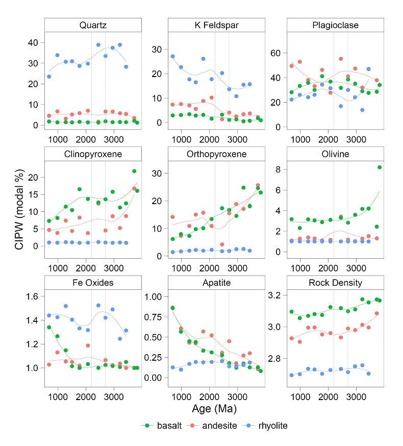
).These element trends can alternatively be presented as shifting mineralogic controls and physical rock properties, such as rock density (Fig. S-9). Modal mineralogy, as inferred from CIPW norms calculated using raw, major-element concentrations (Fig. S-9), also suggest that larger mantle-melt fractions during the Archean may have locally exhausted clinopyroxene and fused more refractory mantle minerals such as orthopyroxene and olivine. These evolving rock properties and estimated modal mineral abundances are thus consistent with decreasing mantle-melt fractions demonstrated by the systematic increase in incompatible versus compatible element log-ratios (Fig. 1), but are based on raw, major-element concentrations.
Figure 1 (a) Schematic spider diagram plotting the composition of the continental crust, normalised to primitive mantle, in relation to isometric-log-ratios (ilr). Numerators and denominators for each ilr-balance are denoted by plus and minus signs, respectively. Each ilr represents a ratio between elements with contrasting compatibility during mantle melting. (b) geochemical evolution of basalt, andesite, and rhyolite magmas based on ilr. Aggregated log-ratio means and loess-curves are colour coded to rock type. Vertical, grey lines represent the Archean-Palaeoproterozoic boundary (2.7–2.2 Ga; Condie and O’Neill, 2010
Condie, K.C., O’Neill, C. (2010) The archean-proterozoic boundary: 500 my of tectonic transition in earth history. American Journal of Science 310, 775–790, doi: 10.2475/09.2010.01.
). Basaltic and andesitic rocks have become incompatible element-rich through time resulting in a negatively sloping ilr-1. Rhyolitic rocks have also become incompatible element-rich (ilr-1), but to a lesser extent and, for some log-ratios (ilr-5–8), yield contrasting trends (positive slopes) that may track the evolving composition of their basaltic to andesitic source. Horizontal lines represent mantle (M; Palme and O’Neill, 2014Palme, H., O’Neill, H.S.C. (2014) Cosmochemical Estimates of Mantle Composition. In: Holland, H., Turekian, K. (Eds.) Treatise on Geochemistry. Elsevier Ltd., 1–38, doi: 10.1016/B978-0-08-095975-7.00201-1.
) and crustal compositions (LW = lower crust; BC = bulk continental crust; Rudnick and Gao, 2003Rudnick, R.L., Gao, S. (2003) Composition of the continental crust. In: Holland, H., Turekian, K. (Eds.) Treatise on Geochemistry, Second Edition. Elsevier, 1–64.
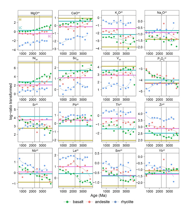
) and are shown for reference. Abbreviations: LILE = large ion lithophile (K, Na, Ba, Sr, Rb, Pb, Cs), LREE = light rare earth element (La, Ce, Pr, Nd); HFSE = high field strength elements (Ti, P, Zr, Hf, Nb, Ta, U, Th); MREE = middle rare earth element (Sm, Eu, Gd); HREE = heavy rare earth element (Tb, Dy, Ho, Er, Yb, Lu, Y); MFE = mantle forming elements (Cr, Ni, Co, Ga, Sc, V).Figure 2 Geochemical evolution of basalt, andesite and rhyolite on an element-by-element basis following a centred log-ratio (clr) approach (Aitchison, 1986
Aitchison, J. (1986) The statistical analysis of compositional data. Chapman & Hall, Ltd. London, UK, 416 pp.
). Vertical, grey lines represent the Archean-Palaeoproterozoic boundary (2.7–2.2 Ga; Condie and O’Neill, 2010Condie, K.C., O’Neill, C. (2010) The archean-proterozoic boundary: 500 my of tectonic transition in earth history. American Journal of Science 310, 775–790, doi: 10.2475/09.2010.01.
). Horizontal lines represent mantle (M; Palme and O’Neill, 2014Palme, H., O’Neill, H.S.C. (2014) Cosmochemical Estimates of Mantle Composition. In: Holland, H., Turekian, K. (Eds.) Treatise on Geochemistry. Elsevier Ltd., 1–38, doi: 10.1016/B978-0-08-095975-7.00201-1.
) and crustal compositions (LW = lower crust; BC = bulk continental crust; Rudnick and Gao, 2003Rudnick, R.L., Gao, S. (2003) Composition of the continental crust. In: Holland, H., Turekian, K. (Eds.) Treatise on Geochemistry, Second Edition. Elsevier, 1–64.
) and are shown for reference. This log-ratio transformation preserves a one-to-one relationship with the original variables, but adding or removing variables changes the absolute value of each clr (see Supplementary Information). Isometric log-ratios (Fig. 1) are not restricted by this constraint and represent the preferred approach for compositional data analysis (Egozcue et al., 2003Egozcue, J., Pawlowsky Glahn, V., Mateu-Figueras, G., Barceló Vidal, C. (2003) Isometric logratio for compositional data analysis. Mathematical Geosciences 35, 279–300, doi: 10.1023/A:1023818214614.
).However, geochemical trends between rock types are only approximately parallel (Figs. 1 and 2). For some element groups (ilr-1–2), basalt and andesite yield diverging, but synced log-ratio patterns during the Archean, suggesting that andesitic rock compositions are more similar to basalt today than they were in the geologic past (Figs. 1 and 2; n.b., except perhaps for the Mesoarchean). Modern andesitic rocks are often interpreted as hybrid melts, produced during mixing of approximately equal proportions of basalt and rhyolite, presumably in upper crustal reservoirs (Rudnick, 1995
Rudnick, R. (1995) Making continental crust. Nature 378, 571–577.
). These mixing models are based, in part, on the bi-modal SiO2 distribution of melt inclusions and rock textures that record disequilibrium conditions between crystals and melt (Reubi and Blundy, 2009Reubi, O., Blundy, J. (2009) A dearth of intermediate melts at subduction zone volcanoes and the petrogenesis of arc andesites. Nature 461, 1269–1273, doi: 10.1038/nature08510.
). Hybridised melt models can reproduce many of the key geochemical features of some Archean andesitic rock suites (Bédard et al., 2013Bédard, J.H., Harris, L.B., Thurston, P.C. (2013) The hunting of the snArc. Precambrian Research 229, 20–48.
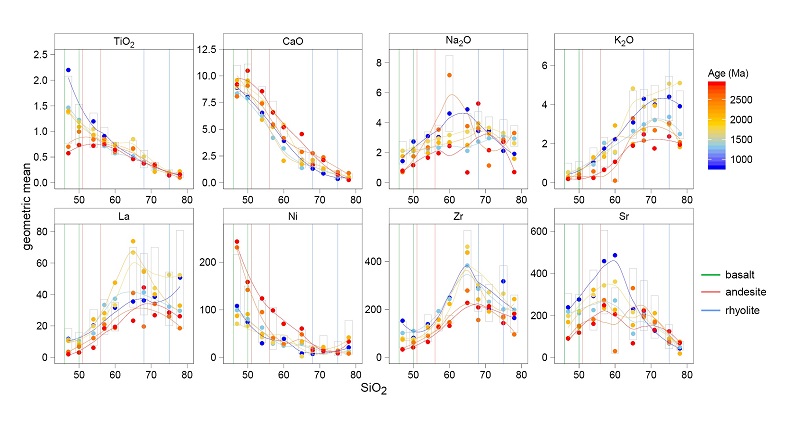
), however, binary mixing between basaltic and rhyolitic rocks are inconsistent with the curved, crystal fraction trends for the multiple time slices presented in Figure 3.Figure 3 Harker diagrams based on the geometric mean of raw SiO2 concentrations. Individual curves are colour coded to age and represent globally averaged, liquid lines of descent for each time slice. Vertical lines represent the inter-quartile range for each rock type. Vertical grey boxes represent the inter-quartile range for each element at any given SiO2 bucket. Overall, ancient crystal fractionation for compatible elements are displaced to lower values at any given SiO2 bucket, consistent with the partial mantle-melt trend based on log-ratios.
Inflexions on these diagrams likely reflect some crystallising mineral phase akin to classic liquid lines of descent (Fig. 3). However, in this case, crystal fractional curves represent globally averaged melting conditions rather than the evolution of a single, co-genetic magma suite (Keller and Schoene, 2012
Keller, C.B., Schoene, B. (2012) Statistical geochemistry reveals disruption in secular lithospheric evolution about 2.5 Gyr ago. Nature 485, 490–493, doi:10.1038/nature11024.
; Keller et al., 2015Keller, C.B., Schoene, B., Barboni, M., Samperton, K.M., Husson, J.M. (2015) Volcanic–plutonic parity and the differentiation of the continental crust. Nature 523, 301, doi: 10.1038/nature14584.
). Compatible elements yield concave-down patterns, which for younger time slices are displaced to lower values at any given SiO2 concentration (Fig. 3). These displaced curves support the partial melting trends described above (Keller and Schoene, 2012Keller, C.B., Schoene, B. (2012) Statistical geochemistry reveals disruption in secular lithospheric evolution about 2.5 Gyr ago. Nature 485, 490–493, doi:10.1038/nature11024.
), but critically, are preserved despite the large range of rock compositions at any given SiO2 interval.Archean rocks with intermediate compositions are relatively rare and, where present, occur as thin layers intercalated with tholeiitic basaltic flows (Furnes et al., 2013
Furnes, H., Dilek, Y., de Wit, M. (2013) Precambrian greenstone sequences represent different ophiolite types. Gondwana Research 27, 649–685, doi: 10.1016/j.gr.2013.06.004.
). These apparent stratigraphic relationships, along with the synced geochemical evolution and curved fractionation trends, tend to suggest that ancient, intermediate rocks represent the fractionated melt products of coeval basaltic magmas. Mixing, or assimilation, with older rocks as is often demonstrated by relatively more sensitive contamination proxies, such as radiogenic isotopes and/or inherited zircon (Allègre and Othman, 1980Allègre, C., Othman, D. (1980) Nd-Sr isotopic relationship in granitoid rocks and continental crust development: A chemical approach to orogenesis. Nature 286, 335–342.
; Hildreth and Moorbath, 1988Hildreth, W., Moorbath, S. (1988) Crustal contributions to arc magmatism in the Andes of Central Chile. Contributions to Mineralogy and Petrology 98, 455–489, doi: 10.1007/BF00372365.
), must have also occurred, but did not significantly disrupt the coupled, geochemical evolution of andesite to its parental basalt at any given age interval.Archean rhyolitic rock compositions, such as the tonalite-trondhjemite-granodiorite (TTG) suite, are also geochemically distinct and, along with lesser basaltic rocks that define narrow, coeval greenstone belts, represent the dominant rock types prior to the Palaeoproterozoic (Furnes et al., 2013
Furnes, H., Dilek, Y., de Wit, M. (2013) Precambrian greenstone sequences represent different ophiolite types. Gondwana Research 27, 649–685, doi: 10.1016/j.gr.2013.06.004.
). The fractionated heavy rare earth element (HREE) TTG signature has been the focus of numerous previous studies and likely reflects a garnet (± hornblende) residue during partial melting of hydrous basaltic rocks that were unlike those at modern, mid-ocean ridges (Bédard, 2006Bédard, J.H. (2006) A catalytic delamination-driven model for coupled genesis of Archaean crust and sub-continental lithospheric mantle. Geochimica et Cosmochimica Acta 70, 1188–1214, doi: 10.1016/j.gca.2005.11.008.
; Martin et al., 2014Martin, H., Moyen, J.-F., Guitreau, M., Blichert-Toft, J., Le Pennec, J.-L. (2014) Why Archaean TTG cannot be generated by MORB melting in subduction zones. Lithos 198–199, 1–13, doi: 10.1016/j.lithos.2014.02.017.
). This unusual trace element behaviour is evident in the current compilation by the anomalous compositions of Meso- to Neoarchean rhyolite (ilr-5, -7, -8; Fig. 1). The data underscore the distinct melting conditions responsible for the TTG suite and their obvious impact on bulk, rhyolitic rock chemistry during the Archean.Post-Archean rocks show a major, composition shift between large-ion lithophile element (LILE)-, high field strength element (HFSE)- and light rare earth element (LREE)-enrichment (Fig. 1; ilr-6–8) in basaltic-andesitic and a corresponding depletion of these elements in similarly-aged rhyolitic magmas. The patterns are clearly defined on an element-by-element basis using log-ratios (Fig. 2), multivariate projections (Figs. S-7 and S-8), and with raw element concentrations (Fig. 3). Post-Archean rocks also tend to be more alkaline in character (Fig. S-5), which coupled with their HFSE- and LILE-rich signature, points to the increasing importance and/or preservation of Phanerozoic-style intra-plate volcanism across the Archean-Proterozoic boundary (2.7–2.2 Ga; Condie and O’Neill, 2010
Condie, K.C., O’Neill, C. (2010) The archean-proterozoic boundary: 500 my of tectonic transition in earth history. American Journal of Science 310, 775–790, doi: 10.2475/09.2010.01.
). The extent to which this signal is influenced by the fragmented, Precambrian rock record, however, is difficult to assess and requires further study (Hawkesworth and Kemp, 2006Hawkesworth, C., Kemp, A. (2006) Evolution of the continental crust. Nature 443, 811–817, doi: 10.1038/nature05191.
). Nevertheless, this trace element signature (Fig. 1; ilr-6–7) forms the basis for most tectonic discrimination diagrams and is distinct from modern, basaltic arc-magmas, which along with rocks comprising many Archean greenstone belts, are generally depleted in HFSE (Pearce, 2008Pearce, J.A. (2008) Geochemical fingerprinting of oceanic basalts with applications to ophiolite classification and the search for Archean oceanic crust. Lithos 100, 14–48, doi: 10.1016/j.lithos.2007.06.016.
). The corresponding HFSE-, LILE- and LREE-poor composition of post-Archean rhyolite seems to suggest that these more differentiated rocks track the evolving composition of their basaltic to andesitic source. As a result, the diverging geochemical patterns of rhyolitic versus basaltic-andesite rocks during the Proterozoic may also reflect, at least in part, the decreasing partial melting trend described above and represent a key geochemical feature of the global, igneous rock record. The Archean-Proterozoic boundary thus represents an important period of Earth’s history that coincided with these modern compositional relationships between crustal building blocks (Figs. 1 and 2).In summary, statistical analysis of global, igneous rock chemistry document the shared geochemical history of basalt, andesite and rhyolite that is synced with decreasing, partial-melting through time (Fig. 1). Diverging, element trends emphasise atypical petrogenetic processes that operated during specific periods of Earth’s history such as: (1) HFSE-rich (ilr-7; Fig. 1) and HREE-poor Archean rhyolitic magmas (i.e. TTG suite; ilr-8; Fig. 1); (2) fractionated Archean andesitic compositions (Figs. 1, 2 and 3); and (3) a major shift towards LREE-, LILE- and HFSE-rich basalt-andesite and corresponding depletion of these elements within coeval rhyolite during the Proterozoic (Figs. 1, 2 and 3). Log-ratios (Egozcue et al., 2003
Egozcue, J., Pawlowsky Glahn, V., Mateu-Figueras, G., Barceló Vidal, C. (2003) Isometric logratio for compositional data analysis. Mathematical Geosciences 35, 279–300, doi: 10.1023/A:1023818214614.
), informed by element behaviour during mantle melting (Fig. 1a), represent a rigorous framework for investigating closed, geochemical data. Future studies will benefit from the addition of high-quality geochemical and geochronologic datasets to the EarthChem Library, particularly for intermediate rock compositions during poorly-represented, but significant periods of Earth’s history such as the Archean-Proterozoic and Neoproterozoic-Cambrian boundaries.top
Acknowledgements
This work was completed under the auspices of the Targeted Geoscience Initiative program and represents ESS contribution (20150469). The hydrogeology group at the GSC is thanked for access to their computing facility. Bruce Kjarsgaard, Eric Grunsky and Vera Pawlowsky-Glahn are thanked for suggestions and discussions that improved an earlier version of the manuscript. John Percival, Peter Cawood and one anonymous reviewer are thanked for thoughtful reviews that improved the clarity of the manuscript.
Editor: Bruce Watson
top
References
Aitchison, J. (1986) The statistical analysis of compositional data. Chapman & Hall, Ltd. London, UK, 416 pp.
 Show in context
 The focus is on estimating the geochemical centre, or central tendency, for each element and rock type through time (Aitchison, 1986; Egozcue et al., 2003).
View in article
Geochemical data, like other forms of compositional data, sum to constant (i.e. closed data) and convey only relative information (Aitchison, 1986).
View in article
Figure 2 Geochemical evolution of basalt, andesite and rhyolite on an element-by-element basis following a centred log-ratio (clr) approach (Aitchison, 1986).
View in article
Allègre, C. (1997) Limitation on the mass exchange between the upper and lower mantle: the evolving convection regime of the Earth. Earth and Planetary Science Letters 150, 1–6.
Show in context The compositional symmetry between the evolved continental crust and the relatively depleted mantle is well documented and helps to define our unique place in the solar system (Allègre, 1997; Taylor and McLennan, 2009).
View in article
Allègre, C., Othman, D. (1980) Nd-Sr isotopic relationship in granitoid rocks and continental crust development: A chemical approach to orogenesis. Nature 286, 335–342.
Show in context Mixing, or assimilation, with older rocks as is often demonstrated by relatively more sensitive contamination proxies, such as radiogenic isotopes and/or inherited zircon (Allègre and Othman, 1980; Hildreth and Moorbath, 1988), must have also occurred, but did not significantly disrupt the coupled, geochemical evolution of andesite to its parental basalt at any given age interval.
View in article
Bédard, J.H. (2006) A catalytic delamination-driven model for coupled genesis of Archaean crust and sub-continental lithospheric mantle. Geochimica et Cosmochimica Acta 70, 1188–1214, doi: 10.1016/j.gca.2005.11.008.
Show in context The fractionated heavy rare earth element (HREE) TTG signature has been the focus of numerous previous studies and likely reflects a garnet (± hornblende) residue during partial melting of hydrous basaltic rocks that were unlike those at modern, mid-ocean ridges (Bédard, 2006; Martin et al., 2014).
View in article
Bédard, J.H., Harris, L.B., Thurston, P.C. (2013) The hunting of the snArc. Precambrian Research 229, 20–48.
Show in context Despite isotopic evidence that suggests the Archean depleted mantle source (at least by 3.8 Ga) was likely similar to today (Vervoort and Blichert-Toft, 1999), the mechanisms driving the production and composition of the continental crust in the geologic past are less understood (Bédard et al., 2013).
View in article
Hybridised melt models can reproduce many of the key geochemical features of some Archean andesitic rock suites (Bédard et al., 2013), however, binary mixing between basaltic and rhyolitic rocks are inconsistent with the curved, crystal fraction trends for the multiple time slices presented in Figure 3.
View in article
Condie, K.C., O’Neill, C. (2010) The archean-proterozoic boundary: 500 my of tectonic transition in earth history. American Journal of Science 310, 775–790, doi: 10.2475/09.2010.01.
Show in context Figure 1 [...] Aggregated log-ratio means and loess-curves are colour coded to rock type. Vertical, grey lines represent the Archean-Palaeoproterozoic boundary (2.7–2.2 Ga; Condie and O’Neill, 2010).
View in article
Figure 2 [...] Vertical, grey lines represent the Archean-Palaeoproterozoic boundary (2.7–2.2 Ga; Condie and O’Neill, 2010).
View in article
Post-Archean rocks also tend to be more alkaline in character (Fig. S-5), which coupled with their HFSE- and LILE-rich signature, points to the increasing importance and/or preservation of Phanerozoic-style intra-plate volcanism across the Archean-Proterozoic boundary (2.7–2.2 Ga; Condie and O’Neill, 2010).
View in article
Egozcue, J., Pawlowsky Glahn, V., Mateu-Figueras, G., Barceló Vidal, C. (2003) Isometric logratio for compositional data analysis. Mathematical Geosciences 35, 279–300, doi: 10.1023/A:1023818214614.
Show in context The focus is on estimating the geochemical centre, or central tendency, for each element and rock type through time (Aitchison, 1986; Egozcue et al., 2003).
View in article
Log-ratios have emerged as one of the preferred approaches for treating such compositional datasets (Egozcue et al., 2003), however, these alternative data treatments can be difficult to interpret in the conventional way, which has limited the application of log-ratio analysis to petrologic problems.
View in article
However, in comparison to interpretations based on raw element concentrations, log-ratios reflect the actual relationships between element groups rather than the spurious effects related to the closed nature of compositional data (Egozcue et al., 2003).
View in article
Isometric log-ratios (ilr-1–8) represent the preferred approach for compositional datasets (Egozcue et al., 2003) and, as defined herein, divide the classic spider diagram into a series of non-overlapping segments (Fig. 1).
View in article
Figure 2 [...] Isometric log-ratios (Fig. 1) are not restricted by this constraint and represent the preferred approach for compositional data analysis (Egozcue et al., 2003).
View in article
Log-ratios (Egozcue et al., 2003), informed by element behaviour during mantle melting (Fig. 1a), represent a rigorous framework for investigating closed, geochemical data.
View in article
Furnes, H., Dilek, Y., de Wit, M. (2013) Precambrian greenstone sequences represent different ophiolite types. Gondwana Research 27, 649–685, doi: 10.1016/j.gr.2013.06.004.
Show in context Archean rocks with intermediate compositions are relatively rare and, where present, occur as thin layers intercalated with tholeiitic basaltic flows (Furnes et al., 2013).
View in article
Archean rhyolitic rock compositions, such as the tonalite-trondhjemite-granodiorite (TTG) suite, are also geochemically distinct and, along with lesser basaltic rocks that define narrow, coeval greenstone belts, represent the dominant rock types prior to the Palaeoproterozoic (Furnes et al., 2013).
View in article
Hawkesworth, C., Kemp, A. (2006) Evolution of the continental crust. Nature 443, 811–817, doi: 10.1038/nature05191.
Show in context This apparent disconnect points to a two-stage, igneous-driven process whereby relatively primitive basaltic magmas are extracted from the mantle and are further differentiated, by re-melting, fractional crystallisation and/or mixing to produce the wide range of igneous rock compositions that are exposed at surface (Hawkesworth and Kemp, 2006).
View in article
The extent to which this signal is influenced by the fragmented, Precambrian rock record, however, is difficult to assess and requires further study (Hawkesworth and Kemp, 2006).
View in article
Herzberg, C., Condie, K., Korenaga, J. (2010) Thermal history of the Earth and its petrological expression. Earth and Planetary Science Letters 292, 79–88, doi: 10.1016/j.epsl.2010.01.022.
Show in context This well-documented pattern is consistent with extensive partial mantle-melting in the geologic past and was possibly driven by hotter, Archean mantle temperatures (Herzberg et al., 2010; Keller and Schoene, 2012).
View in article
Hildreth, W., Moorbath, S. (1988) Crustal contributions to arc magmatism in the Andes of Central Chile. Contributions to Mineralogy and Petrology 98, 455–489, doi: 10.1007/BF00372365.
Show in context Mixing, or assimilation, with older rocks as is often demonstrated by relatively more sensitive contamination proxies, such as radiogenic isotopes and/or inherited zircon (Allègre and Othman, 1980; Hildreth and Moorbath, 1988), must have also occurred, but did not significantly disrupt the coupled, geochemical evolution of andesite to its parental basalt at any given age interval.
View in article
Keller, C.B., Schoene, B. (2012) Statistical geochemistry reveals disruption in secular lithospheric evolution about 2.5 Gyr ago. Nature 485, 490–493, doi: 10.1038/nature11024.
Show in context Weighted bootstrap re-sampling of the data (weighted inversely to age) was used to minimise the effect of unevenly distributed crystallisation ages (Fig. S-6), which are inherent to the punctuated, igneous rock record (Keller and Schoene, 2012).
View in article
This well-documented pattern is consistent with extensive partial mantle-melting in the geologic past and was possibly driven by hotter, Archean mantle temperatures (Herzberg et al., 2010; Keller and Schoene, 2012).
View in article
However, in this case, crystal fractional curves represent globally averaged melting conditions rather than the evolution of a single, co-genetic magma suite (Keller and Schoene, 2012; Keller et al., 2015).
View in article
These displaced curves support the partial melting trends described above (Keller and Schoene, 2012), but critically, are preserved despite the large range of rock compositions at any given SiO2 concentration.
View in article
Keller, C.B., Schoene, B., Barboni, M., Samperton, K.M., Husson, J.M. (2015) Volcanic–plutonic parity and the differentiation of the continental crust. Nature 523, 301, doi: 10.1038/nature14584.
Show in context However, in this case, crystal fractional curves represent globally averaged melting conditions rather than the evolution of a single, co-genetic magma suite (Keller and Schoene, 2012; Keller et al., 2015).
View in article
Le Bas, M., Le Maitre, R., Steckeisen, A., Zanettin, B. (1986) The construction of the total alkali–silica chemical classification of volcanic rocks. Journal of Petroleum Science and Engineering 27, 745–750.
Show in context Precambrian samples (≥541 Ma; n = 66,739) were then discretised into basaltic, andesitic and rhyolitic compositions based on the Total Alkali Silica (Le Bas et al., 1986) and Pearce (Pearce, 1996) classification diagrams (Figs. S-4 and S-5).
View in article
Lee, C.-T.A., Bachmann, O. (2014) How important is the role of crystal fractionation in making intermediate magmas? Insights from Zr and P systematics. Earth and Planetary Science Letters 393, 266–274, doi: 10.1016/j.epsl.2014.02.044.
Show in context Whether these ancient intermediate rock compositions represent primary mantle melts, mixing between differentiated basaltic and rhyolitic melts and/or are crystal fractionation products of basaltic magmas, however, remains controversial (Reubi and Blundy, 2009; Lee and Bachmann, 2014).
View in article
Martin, H., Moyen, J.-F., Guitreau, M., Blichert-Toft, J., Le Pennec, J.-L. (2014) Why Archaean TTG cannot be generated by MORB melting in subduction zones. Lithos 198–199, 1–13, doi: 10.1016/j.lithos.2014.02.017.
Show in context The fractionated heavy rare earth element (HREE) TTG signature has been the focus of numerous previous studies and likely reflects a garnet (± hornblende) residue during partial melting of hydrous basaltic rocks that were unlike those at modern, mid-ocean ridges (Bédard, 2006; Martin et al., 2014).
View in article
Palme, H., O’Neill, H.S.C. (2014) Cosmochemical Estimates of Mantle Composition. In: Holland, H., Turekian, K. (Eds.) Treatise on Geochemistry. Elsevier Ltd., 1–38, doi: 10.1016/B978-0-08-095975-7.00201-1.
Show in context Figure 1 [...] Horizontal lines represent mantle (M; Palme and O’Neill, 2014) and crustal compositions (LW = lower crust; BC = bulk continental crust; Rudnick and Gao, 2003) and are shown for reference.
View in article
Figure 2 [...] Horizontal lines represent mantle (M; Palme and O’Neill, 2014) and crustal compositions (LW = lower crust; BC = bulk continental crust; Rudnick and Gao, 2003) and are shown for reference.
View in article
Pearce, J. (1996) A users guide to basalt discrimination diagrams. In: Pearce, J., Wyman, D. (Eds.) Geological Association of Canada, Short Course Notes. Geological Association of Canada, 79–113.
Show in context Precambrian samples (≥541 Ma; n = 66,739) were then discretised into basaltic, andesitic and rhyolitic compositions based on the Total Alkali Silica (Le Bas et al., 1986) and Pearce (Pearce, 1996) classification diagrams (Figs. S-4 and S-5).
View in article
Pearce, J.A. (2008) Geochemical fingerprinting of oceanic basalts with applications to ophiolite classification and the search for Archean oceanic crust. Lithos 100, 14–48, doi: 10.1016/j.lithos.2007.06.016.
Show in context Slope changes on these classic diagrams, which can be further reduced to ratios (or log-ratios in this case) between elements of contrasting compatibility (incompatible versus compatible elements), reflect igneous differentiation processes such as the degree of partial melting and/or fractional crystallisation (Pearce, 2008).
View in article
These smaller segments reflect key petrogenetic indicators such as large ion lithophile element (LILE)- and high field strength element (HFSE)-enrichment (ilr-6 and ilr-7, respectively), and can also be constructed to reproduce commonly used ratios, such as Sm/Yb, which monitor the influence of key mineral phases (e.g., garnet) during melting (ilr-8; Pearce, 2008).
View in article
Nevertheless, this trace element signature (Fig. 1; ilr-6–7) forms the basis for most tectonic discrimination diagrams and is distinct from modern, basaltic arc-magmas, which along with rocks comprising many Archean greenstone belts, are generally depleted in HFSE (Pearce, 2008).
View in article
R Core Team (2015) R: A language and environment for statistical computing. R Foundation for Statistical Computing, Vienna, Austria. URL https://www.R-project.org/.
Show in context Data processing and figures can also be reproduced using the free, open source R software environment (R Core Team, 2015) and code available from the corresponding author.
View in article
Reubi, O., Blundy, J. (2009) A dearth of intermediate melts at subduction zone volcanoes and the petrogenesis of arc andesites. Nature 461, 1269–1273, doi: 10.1038/nature08510.
Show in context Whether these ancient intermediate rock compositions represent primary mantle melts, mixing between differentiated basaltic and rhyolitic melts and/or are crystal fractionation products of basaltic magmas, however, remains controversial (Reubi and Blundy, 2009; Lee and Bachmann, 2014).
View in article
These mixing models are based, in part, on the bi-modal SiO2 distribution of melt inclusions and rock textures that record disequilibrium conditions between crystals and melt (Reubi and Blundy, 2009).
View in article
Rudnick, R. (1995) Making continental crust. Nature 378, 571–577.
Show in context New continental crust, generated today at convergent and intra-plate settings, is predominately basaltic and thus contrasts with the andesitic composition of the bulk continental crust (Rudnick, 1995; Taylor and McLennan, 1995).
View in article
Modern andesitic rocks are often interpreted as hybrid melts, produced during mixing of approximately equal proportions of basalt and rhyolite, presumably in upper crustal reservoirs (Rudnick, 1995).
View in article
Rudnick, R.L., Gao, S. (2003) Composition of the continental crust. In: Holland, H., Turekian, K. (Eds.) Treatise on Geochemistry, Second Edition. Elsevier, 1–64.
Show in context Figure 1 [...] Horizontal lines represent mantle (M; Palme and O’Neill, 2014) and crustal compositions (LW = lower crust; BC = bulk continental crust; Rudnick and Gao, 2003) and are shown for reference.
View in article
Figure 2 [...] Horizontal lines represent mantle (M; Palme and O’Neill, 2014) and crustal compositions (LW = lower crust; BC = bulk continental crust; Rudnick and Gao, 2003) and are shown for reference.
View in article
Taylor, S., McLennan, S. (2009) Planetary Crusts. Cambridge University Press, Cambridge, 404 pp.
Show in context The compositional symmetry between the evolved continental crust and the relatively depleted mantle is well documented and helps to define our unique place in the solar system (Allègre, 1997; Taylor and McLennan, 2009).
View in article
Taylor, S., McLennan, S. (1995) The geochemical evolution of the continental crust. Reviews of Geophysics and Space Physics 33, 241–265.
Show in context New continental crust, generated today at convergent and intra-plate settings, is predominately basaltic and thus contrasts with the andesitic composition of the bulk continental crust (Rudnick, 1995; Taylor and McLennan, 1995).
View in article
van Buuren, S., Groothuis-Oudshoorn, K. (2011) mice: Multivariate Imputation by Chained Equations in R. Journal of Statistical Software 45, 1-67.
Show in context Log-ratio analysis requires complete datasets and thus, in this case, missing values for elements with minor to moderate degrees of missingness (typically 10–30 % missing) were replaced using column-wise multivariate imputation by chained equations (van Buuren and Groothuis-Oudshoorn, 2011).
View in article
Vervoort, J.D., Blichert-Toft, J. (1999) Evolution of the depleted mantle: Hf isotope evidence from juvenile rocks through time. Geochimica et Cosmochimica Acta 63, 533–556, doi: 10.1016/S0016-7037(98)00274-9.
Show in context Despite isotopic evidence that suggests the Archean depleted mantle source (at least by 3.8 Ga) was likely similar to today (Vervoort and Blichert-Toft, 1999), the mechanisms driving the production and composition of the continental crust in the geologic past are less understood (Bédard et al., 2013).
View in article
top
Supplementary Information
Supplementary Methods
Data compilation and missing values. All data processing and interpretation was completed in R (R Core Team, 2015
R Core Team (2015) R: A language and environment for statistical computing. R Foundation for Statistical Computing, Vienna, Austria. URL https://www.R-project.org/.
). Code and processed datasets are available from the corresponding author. Igneous rock geochemistry and ages were downloaded and compiled from the EarthChem Library (www.earthchem.org). Selected Precambrian (≥541 Ma) samples (n = 66,739) contained a relatively large proportion of missing values, particularly for some elements. Log-ratio transformations, the preferred approach for compositional data (discussed below) and, many multivariate statistical methods, require complete datasets (Palarea-Albaladejo and Martín-Fernández, 2015Palarea-Albaladejo, J., Martín-Fernández, J.A. (2015) zCompositions — R package for multivariate imputation of left-censored data under a compositional approach. Chemometrics and Intelligent Laboratory Systems 143, 85–96, doi: 10.1016/j.chemolab.2015.02.019.
). In this case, missing values are likely due to a combination of element concentrations that were below the analytical detection limit, elements that were not collected as part of that particular analytical suite and/or potentially a variety of other unknown reasons. Unfortunately, differentiating between these different types of missing values was impractical, if not impossible, for such a large and diverse dataset and thus all missing values were treated similarly.Samples (rows) and elements (columns) with greater than 50 % missing values were removed prior to imputing the remaining missing values using column-wise multivariate imputation by chained equations (van Buuren and Groothuis-Oudshoorn, 2011
van Buuren, S., Groothuis-Oudshoorn, K. (2011) mice: Multivariate Imputation by Chained Equations in R. Journal of Statistical Software 45, 1-67.
). Missing values comprised between 10 and 30 % for most elements. Other imputation approaches are available (Palarea-Albaladejo and Martín-Fernández, 2015Palarea-Albaladejo, J., Martín-Fernández, J.A. (2015) zCompositions — R package for multivariate imputation of left-censored data under a compositional approach. Chemometrics and Intelligent Laboratory Systems 143, 85–96, doi: 10.1016/j.chemolab.2015.02.019.
) and the selected method, particular for elements with a relatively large proportion of missing values, is pertinent to the secular geochemical trends that are the focus of the current study. Ideally, imputed concentrations are realistic and reflect a value that could have been observed had it not been missing. The plausibility of imputed values was checked qualitatively, and on a univariate basis, by comparing the distribution of five imputation iterations with the kernel density distribution of complete-cases (Figs. S-2 and S-3). For most elements, the imputed distributions compare well with the actually observed distribution (Fig. S-2a), suggesting that imputed values are geologically reasonable. Whether these missing values shifted the centre of the data, which is the focus herein, was also tested by comparing boxplot distributions before and after imputation for all elements (Fig. 3).Figure S-1 Geographic distribution of Precambrian EarthChem Library samples included within the present study.
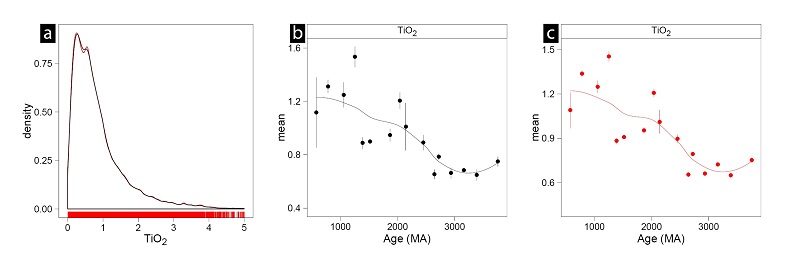
Figure S-2 (a) Complete cases (black) versus imputed (red) kernel density distributions for TiO2. (b-c) Overall, the imputed values are realistic and do not affect the secular trends that are the focus herein. Error-bars are reported as 2 × standard error of the mean.
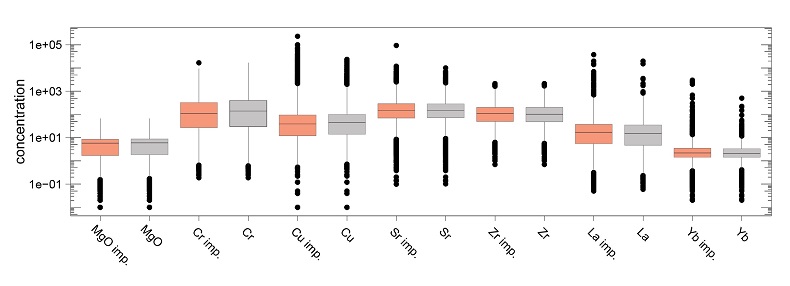
Figure S-3 Boxplot distributions for complete-cases (black) versus the imputed dataset (dots represent outliers). Imputed values do not significantly affect the central tendency for elements that possess between 10 and 50 % missing values (left to right).
The imputed dataset was then discretised into basaltic, andesitic and rhyolitic compositions based on the classic TAS (Le Bas et al., 1986
Le Bas, M., Le Maitre, R., Steckeisen, A., Zanettin, B. (1986) The construction of the total alkali–silica chemical classification of volcanic rocks. Journal of Petroleum Science and Engineering 27, 745–750.
) and Pearce (Pearce, 1996Pearce, J. (1996) A users guide to basalt discrimination diagrams. In: Pearce, J., Wyman, D. (Eds.) Geological Association of Canada, Short Course Notes. Geological Association of Canada, 79–113.
) classification diagrams. Samples that were not correctly classified in both diagrams were excluded from the following statistical analysis. This combined classification approach, which is based on mobile- and least-mobile elements, reduces the impact of metasomatised samples and identifies unrealistic rock compositions (Figs. S-4 and S-5). Metamorphosed and hydrothermally altered rocks represent a significant proportion of the dataset (n = 8,839) and suggest that identifying least-metasomatised samples (n = 18,246) is particularly important for the Precambrian igneous rock record. Normative mineralogy was calculated for this least-altered sample-set using major element concentrations on a volatile-free basis (Guzman, 2015Guzman, R. (2015) NORRRM: Geochemical Toolkit for R. https://cran.r-project.org/web/packages/NORRRM/index.html.
).Figure S-4 TAS (left) and Pearce (right) rock classification diagrams colour coded to rock type. Only the first 100 (out of 10,000) re-sampled datasets are shown for clarity. Rock names: 1 = picro-basalt; 2 = basalt; 3 = basaltic andesite; 4 = andesite; 5 = dacite; 6 = rhyolite; 7 = basanite; 8 = trachy-basalt; 9 = basaltic trachy-andesite; 10 = trachyte; 12 = phonotephrite; 13 = tephriphonolite; 14 = phonolite; 15 = foidite.
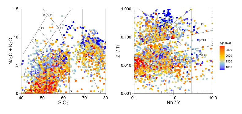
Figure S-5 TAS (left) and Pearce (right) rock classification diagrams colour coded to age. Only the first 100 (out of 10,000) re-sampled datasets are shown for clarity. The tendency for modern rock types to be alkali element-rich is clear even within this simple data projection. Rock names: 1 = picro-basalt; 2 = basalt; 3 = basaltic andesite; 4 = andesite; 5 = dacite; 6 = rhyolite; 7 = basanite; 8 = trachy-basalt; 9 = basaltic trachy-andesite; 10 = trachyte; 12 = phonotephrite; 13 = tephriphonolite; 14 = phonolite; 15 = foidite.
Weighted bootstrap re-sampling. The rock record is unevenly distributed in space and time due to the combined effects of igneous processes and preservation bias (Cawood et al., 2013
Cawood, P., Hawkesworth, C., Dhuime, B. (2013) The continental record and the generation of continental crust. Geological Society of America Bulletin 125, 14–32.
). A significant proportion of the EarthChem database also contains poorly-defined ages that contribute to the sample clustering at specific ages (e.g., 3.1 Ga; Fig. S-6a). Herein the effect of this uneven distribution on secular geochemical trends was evaluated with weighted bootstrap re-sampling (Keller and Schoene, 2012Keller, C.B., Schoene, B. (2012) Statistical geochemistry reveals disruption in secular lithospheric evolution about 2.5 Gyr ago. Nature 485, 490–493, doi: 10.1038/nature11024.
). Samples were weighted inversely proportional to age using kernel-based density estimations (Duong, 2007Duong, T. (2007) ks: Kernel density estimation and kernel discriminant analysis for multivariate data in R. Journal of Statistical Software 21, 1–16.
). Subsets of these weighted samples (n = 100) were then discretised into age groups using K-means clustering (Bivand, 2015Bivand, R. (2015) classInt: Choose Univariate Class Intervals. https://cran.r-project.org/web/packages/classInt/index.html.
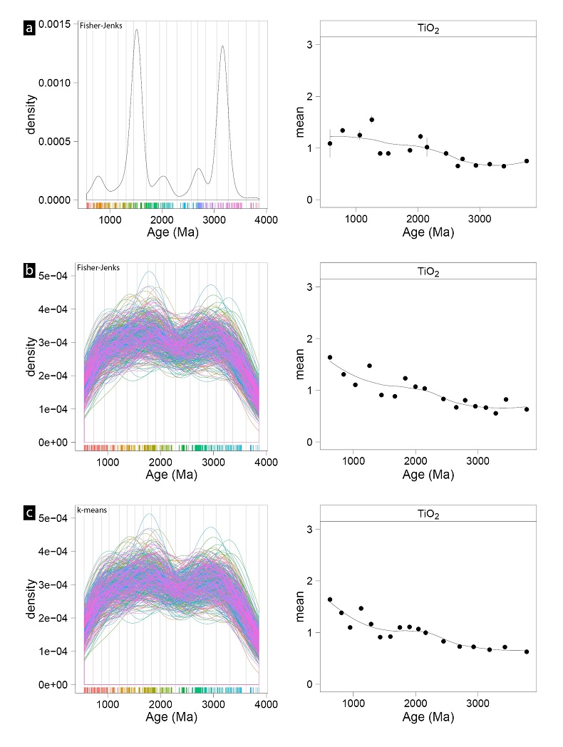
). This process was repeated 10,000 times prior to log-transforming the data and calculating means and standard errors for each variable by rock- and age-group. In general, the re-sampled data resulted in more uniform, posterior age distributions due to the reduced influence of peak crystallisation ages (Fig. S-6). Although qualitative, the re-sampled data appear to produce a close-fit with the geochemical trends defined by the original data, suggesting that the uneven distribution of crystallisation ages or the selected age-groupings do not impact the overall conclusions discussed herein (Fig. S-6). Nevertheless, re-sampled data were used for all further statistical processing to limit the influence of those samples with poorly-defined ages.Figure S-6 (a) Original data distribution and secular TiO2 trend fitted with loess. Data clustering is due to the uneven distribution of the igneous rock record and false age-peaks related to poorly-defined ages within the EarthChem library. The impact of this punctuated igneous rock record was minimised by weighted bootstrap re-sampling (weighted inversely to age density; see text for discussion). Vertical lines are age buckets defined by the Fisher-Jenks method. Rug plots are colour coded to age bucket. (b–c) Kernel density distributions for the first 1,000 re-sampled iterations (out of 10,000; density curves are colour coded to iteration number) and secular TiO2 trends fitted with loess. Vertical lines are age buckets defined by the Fisher-Jenks and K-means methods, respectively. Rug plots colour coded to age bucket. Overall, re-sampled data for even this relatively small-number of iterations closely approximates the trend defined by the original dataset.
Log-ratio transformations. Element concentrations, like other compositional data, sum to a constant and have unique statistical properties (Aitchison, 1986
Aitchison, J. (1986) The statistical analysis of compositional data. Chapman & Hall, Ltd. London, UK, 416 pp.
). Log-ratio approaches (i.e. logarithms of ratios of compositional parts) provide a framework for handling compositional data and work by transforming a D-part composition, known as the simplex (x = [x1, x2,…,xD]), into multi-dimensional real-space (Aitchison, 1986Aitchison, J. (1986) The statistical analysis of compositional data. Chapman & Hall, Ltd. London, UK, 416 pp.
). Transformed data are then analysed in the conventional way.Herein two log-ratio transformations were employed. The centred log-ratio (clr) approach transforms a D-part composition into a D-real-vector (Aitchison, 1986
Aitchison, J. (1986) The statistical analysis of compositional data. Chapman & Hall, Ltd. London, UK, 416 pp.
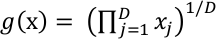
). Each clr can be considered as a compositional coordinate and is calculated by dividing each compositional vector x by the geometric mean g(x) and then taking the logarithms:Eq. S-1
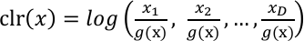
Where
Calculated clr coordinates possess a one-to-one relationship with the original variables (Fig. 2), but are sub-compositionally incoherent (i.e. adding or removing variables changes the calculated clrs). Isometric log-ratio (ilr) transformations provide an alternate representation of compositional data that generates D-1 coordinates and an orthogonal system of axes in real space that facilitate further statistical analysis (Egozcue et al., 2003
Egozcue, J., Pawlowsky Glahn, V., Mateu-Figueras, G., Barceló Vidal, C. (2003) Isometric logratio for compositional data analysis. Mathematical Geosciences 35, 279–300, doi: 10.1023/A:1023818214614.
). Orthonormal ilr-coordinates can be defined by a sequential binary partition (SBP) using the concept of balances (Egozcue et al., 2003Egozcue, J., Pawlowsky Glahn, V., Mateu-Figueras, G., Barceló Vidal, C. (2003) Isometric logratio for compositional data analysis. Mathematical Geosciences 35, 279–300, doi: 10.1023/A:1023818214614.
; Van Der Boogaart and Tolosana-Delgado, 2006Van Der Boogaart, K.G., Tolosana-Delgado, R. (2006) Compositional data analysis with “R” and the package “compositions.” Geological Society London, Special Publication 264, 119–127, doi: 10.1144/GSL.SP.2006.264.01.09.
; Pawlowsky-Glahn and Egozcue, 2011Pawlowsky-Glahn, V., Egozcue, J. (2011) Exploring Compositional Data with the CoDa-Dendrogram. Austrian Journal of Statistics 40, 103–113.
). First, a compositional vector is divided into two, non-overlapping groups of parts. Each group is further divided until all groups contain a single part (Fig. 1). This process results in a series of partitions that correspond to D-1 ilr-coordinates, which for the jth balance is defined as:Eq. S-2
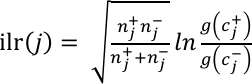
Where nj+ and nj- are the number of parts in the numerator and denominator, respectively, in the jth row of the sequential binary partition; g(cj+) and g(cj-) are the geometric mean of the components in the numerator and denominator, respectively.
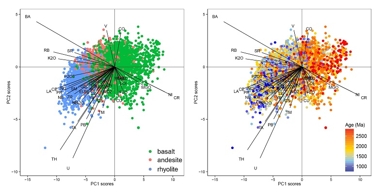
Balances were simplified by splitting elements into groups prior to log-ratio transformations. Element groupings correspond to known geochemical behaviour and were guided, in this specific case, by clusters of elements following robust Principal Component Analysis (PCA; Figs. S-7 and S-8; Templ et al., 2011
Templ, M., Hron, K., Filzmoser, P. (2011) robCompositions: an R-package for robust statistical analysis of compositional data. In: Pawlowsky-Glahn, V., Buccianti, A. (Eds.) Compositional Data Analysis. Theory and Applications. John Wiley & Sons, Chichester (UK), 341–355.
). Each element group is defined as: (1) large ion lithophile elements (LILE) = K, Na, Ba, Sr, Rb, Pb, Cs; (2) light rare earth elements (LREE) = La, Ce, Pr, Nd; (3) high field strength elements (HFSE) = Ti, P, Zr, Hf, Nb, Ta, U, Th; (3) middle rare earth element (MREE) = Sm, Eu, Gd; (4) heavy rare earth elements (HREE) = Tb, Dy, Ho, Er, Yb, Lu, Y; (5) Al-Si; (6) chalcophile elements = Cu, Zn; (7) Mg, Fe, Ca, Mn; and (8) mantle forming elements (MFE) = Cr, Ni, Co, Ga, Sc, V.Figure S-7 Robust principal component analysis (Templ et al., 2011
Templ, M., Hron, K., Filzmoser, P. (2011) robCompositions: an R-package for robust statistical analysis of compositional data. In: Pawlowsky-Glahn, V., Buccianti, A. (Eds.) Compositional Data Analysis. Theory and Applications. John Wiley & Sons, Chichester (UK), 341–355.
) colour coded to rock type (left) and age (right) using the original variables. The first principal component represents an effective proxy for rock type. Only the first 100 (out of 10,000) re-sampled datasets are shown for clarity.Figure S-8 Robust principal component analysis (Templ et al., 2011
Templ, M., Hron, K., Filzmoser, P. (2011) robCompositions: an R-package for robust statistical analysis of compositional data. In: Pawlowsky-Glahn, V., Buccianti, A. (Eds.) Compositional Data Analysis. Theory and Applications. John Wiley & Sons, Chichester (UK), 341–355.
) colour coded to rock type (left) and age (right) using element groups. The similarities between this projection and principal component analysis using the original elements (Fig. S-7) suggests that reducing the number of variables does not impact the results. Only the first 1,000 (out of 10,000) re-sampled datasets are shown for clarity.Figure S-9 Normative mineralogy (modal %) based on CIPW calculations using raw major element concentrations in R (Guzman, 2015
Guzman, R. (2015) NORRRM: Geochemical Toolkit for R. https://cran.r-project.org/web/packages/NORRRM/index.html.
). Vertical, grey lines represent the Archean-Palaeoproterozoic boundary (2.7–2.2 Ga; Condie and O’Neill, 2010Condie, K.C., O’Neill, C. (2010) The archean-proterozoic boundary: 500 my of tectonic transition in earth history. American Journal of Science 310, 775–790, doi: 10.2475/09.2010.01.
). Extensive partial melting during the Archean exhausted clinopyroxene and fused more refractory minerals such as orthopyroxene and olivine.Element groups were then ordered according to their compatibility during mantle melting (Fig. 1). The order is equivalent to classic, multi-element diagrams, or spider plots (Hofmann, 1988
Hofmann, A. (1988) Chemical differentiation of the Earth: The relationship between mantle, continental crust, and oceanic crust. Earth and Planetary Science Letters 90, 297–314, doi: 10.1016/0012-821X(88)90132-X.
; Pearce, 2008Pearce, J.A. (2008) Geochemical fingerprinting of oceanic basalts with applications to ophiolite classification and the search for Archean oceanic crust. Lithos 100, 14–48, doi: 10.1016/j.lithos.2007.06.016.
). As a result, each ilr can be interpreted in the conventional petrological sense. Simply put, a positive ilr suggests that the geometric mean of the numerator is greater than the geometric mean of the denominator. For ilrs that represent ratios of incompatible and compatible elements through time (Fig. 1b), an increasing ilr suggests that these rocks have become more incompatible element rich through time. The geologic significance of each ilr is displayed graphically in Figure 1a.Supplementary Information References
Aitchison, J. (1986) The statistical analysis of compositional data. Chapman & Hall, Ltd. London, UK, 416 pp.
Show in context Element concentrations, like other compositional data, sum to a constant and have unique statistical properties (Aitchison, 1986).
View in Supplementary Information
Log-ratio approaches (i.e. logarithms of ratios of compositional parts) provide a framework for handling compositional data and work by transforming a D-part composition, known as the simplex (x = [x1, x2,…,xD]), into multi-dimensional real-space (Aitchison, 1986).
View in Supplementary Information
The centred log-ratio (clr) approach transforms a D-part composition into a D-real-vector (Aitchison, 1986).
View in Supplementary Information
Bivand, R. (2015) classInt: Choose Univariate Class Intervals. https://cran.r-project.org/web/packages/classInt/index.html.
Show in context Subsets of these weighted samples (n = 100) were then discretised into age groups using K-means clustering (Bivand, 2015).
View in Supplementary Information
Cawood, P., Hawkesworth, C., Dhuime, B. (2013) The continental record and the generation of continental crust. Geological Society of America Bulletin 125, 14–32.
Show in context The rock record is unevenly distributed in space and time due to the combined effects of igneous processes and preservation bias (Cawood et al., 2013).
View in Supplementary Information
Condie, K.C., O’Neill, C. (2010) The archean-proterozoic boundary: 500 my of tectonic transition in earth history. American Journal of Science 310, 775–790, doi: 10.2475/09.2010.01.
Show in context Figure S-9 [...] Vertical, grey lines represent the Archean-Palaeoproterozoic boundary (2.7–2.2 Ga; Condie and O’Neill, 2010).
View in Supplementary Information
Duong, T. (2007) ks: Kernel density estimation and kernel discriminant analysis for multivariate data in R. Journal of Statistical Software 21, 1–16.
Show in context Samples were weighted inversely proportional to age using kernel-based density estimations (Duong, 2007).
View in Supplementary Information
Egozcue, J., Pawlowsky Glahn, V., Mateu-Figueras, G., Barceló Vidal, C. (2003) Isometric logratio for compositional data analysis. Mathematical Geosciences 35, 279–300, doi: 10.1023/A:1023818214614.
Show in context Isometric log-ratio (ilr) transformations provide an alternate representation of compositional data that generates D-1 coordinates and an orthogonal system of axes in real space that facilitate further statistical analysis (Egozcue et al., 2003).
View in Supplementary Information
Orthonormal ilr-coordinates can be defined by a sequential binary partition (SBP) using the concept of balances (Egozcue et al., 2003; Van Der Boogaart and Tolosana-Delgado, 2006; Pawlowsky-Glahn and Egozcue, 2011).
View in Supplementary Information
Guzman, R. (2015) NORRRM: Geochemical Toolkit for R. https://cran.r-project.org/web/packages/NORRRM/index.html.
Show in context Normative mineralogy was calculated for this least-altered sample-set using major element concentrations on a volatile-free basis (Guzman, 2015).
View in Supplementary Information
Figure S-9 Normative mineralogy (modal %) based on CIPW calculations using raw major element concentrations in R (Guzman, 2015).
View in Supplementary Information
Hofmann, A. (1988) Chemical differentiation of the Earth: The relationship between mantle, continental crust, and oceanic crust. Earth and Planetary Science Letters 90, 297–314, doi: 10.1016/0012-821X(88)90132-X.
Show in context The order is equivalent to classic, multi-element diagrams, or spider plots (Hofmann, 1988; Pearce, 2008).
View in Supplementary Information
Keller, C.B., Schoene, B. (2012) Statistical geochemistry reveals disruption in secular lithospheric evolution about 2.5 Gyr ago. Nature 485, 490–493, doi: 10.1038/nature11024.
Show in context Herein the effect of this uneven distribution on secular geochemical trends was evaluated with weighted bootstrap re-sampling (Keller and Schoene, 2012).
View in Supplementary Information
Le Bas, M., Le Maitre, R., Steckeisen, A., Zanettin, B. (1986) The construction of the total alkali–silica chemical classification of volcanic rocks. Journal of Petroleum Science and Engineering 27, 745–750.
Show in context The imputed dataset was then discretised into basaltic, andesitic and rhyolitic compositions based on the classic TAS (Le Bas et al., 1986) and Pearce (Pearce, 1996) classification diagrams.
View in Supplementary Information
Palarea-Albaladejo, J., Martín-Fernández, J.A. (2015) zCompositions — R package for multivariate imputation of left-censored data under a compositional approach. Chemometrics and Intelligent Laboratory Systems 143, 85–96, doi: 10.1016/j.chemolab.2015.02.019.
Show in context Log-ratio transformations, the preferred approach for compositional data (discussed below) and, many multivariate statistical methods, require complete datasets (Palarea-Albaladejo and Martín-Fernández, 2015).
View in Supplementary Information
Other imputation approaches are available (Palarea-Albaladejo and Martín-Fernández, 2015) and the selected method, particular for elements with a relatively large proportion of missing values, is pertinent to the secular geochemical trends that are the focus of the current study.
View in Supplementary Information
Pawlowsky-Glahn, V., Egozcue, J. (2011) Exploring Compositional Data with the CoDa-Dendrogram. Austrian Journal of Statistics 40, 103–113.
Show in context Orthonormal ilr-coordinates can be defined by a sequential binary partition (SBP) using the concept of balances (Egozcue et al., 2003; Van Der Boogaart and Tolosana-Delgado, 2006; Pawlowsky-Glahn and Egozcue, 2011).
View in Supplementary Information
Pearce, J. (1996) A users guide to basalt discrimination diagrams. In: Pearce, J., Wyman, D. (Eds.) Geological Association of Canada, Short Course Notes. Geological Association of Canada, 79–113.
Show in context The imputed dataset was then discretised into basaltic, andesitic and rhyolitic compositions based on the classic TAS (Le Bas et al., 1986) and Pearce (Pearce, 1996) classification diagrams.
View in Supplementary Information
Pearce, J.A. (2008) Geochemical fingerprinting of oceanic basalts with applications to ophiolite classification and the search for Archean oceanic crust. Lithos 100, 14–48, doi: 10.1016/j.lithos.2007.06.016.
Show in context The order is equivalent to classic, multi-element diagrams, or spider plots (Hofmann, 1988; Pearce, 2008).
View in Supplementary Information
R Core Team (2015) R: A language and environment for statistical computing. R Foundation for Statistical Computing, Vienna, Austria. URL https://www.R-project.org/.
Show in context All data processing and interpretation was completed in R (R Core Team, 2015).
View in Supplementary Information
Templ, M., Hron, K., Filzmoser, P. (2011) robCompositions: an R-package for robust statistical analysis of compositional data. In: Pawlowsky-Glahn, V., Buccianti, A. (Eds.) Compositional Data Analysis. Theory and Applications. John Wiley & Sons, Chichester (UK), 341–355.
Show in context Element groupings correspond to known geochemical behaviour and were guided, in this specific case, by clusters of elements following robust Principal Component Analysis (PCA; Figs. S-7 and S-8; Templ et al., 2011).
View in Supplementary Information
Figure S-7 Robust principal component analysis (Templ et al., 2011) colour coded to rock type (left) and age (right) using the original variables.
View in Supplementary Information
Figure S-8 Robust principal component analysis (Templ et al., 2011) colour coded to rock type (left) and age (right) using element groups.
View in Supplementary Information
van Buuren, S., Groothuis-Oudshoorn, K. (2011) mice: Multivariate Imputation by Chained Equations in R. Journal of Statistical Software 45, 1-67.
Show in context Samples (rows) and elements (columns) with greater than 50 % missing values were removed prior to imputing the remaining missing values using column-wise multivariate imputation by chained equations (van Buuren and Groothuis-Oudshoorn, 2011).
View in Supplementary Information
Van Der Boogaart, K.G., Tolosana-Delgado, R. (2006) Compositional data analysis with “R” and the package “compositions.” Geological Society London, Special Publication 264, 119–127, doi: 10.1144/GSL.SP.2006.264.01.09.
Show in context Orthonormal ilr-coordinates can be defined by a sequential binary partition (SBP) using the concept of balances (Egozcue et al., 2003; Van Der Boogaart and Tolosana-Delgado, 2006; Pawlowsky-Glahn and Egozcue, 2011).
View in Supplementary Information