


A novel carbon cycle turbulence index identifies environmental and ecological perturbations
Affiliations | Corresponding Author | Cite as | Funding informationPublished by the European Association of Geochemistry
under Creative Commons License CC BY-NC-ND 4.0
Keywords: carbon isotope, extinction rates, Permian-Triassic transition, the industrial revolution, Phanerozoic, Suess effect


- Share this article


-
Article views:2,465Cumulative count of HTML views and PDF downloads.
- Download Citation
- Rights & Permissions

top
Abstract
Figures
 Figure 1 δ13Ccarb database (Cramer and Jarvis, 2020) and calculated CTindex values across the last 1,000 Myr, combined with calculated extinction rates through the Phanerozoic (from the palaeobiology database; http://www.paleobiodb.org/; Kocsis et al., 2019). | 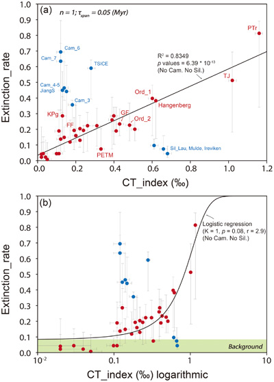 Figure 2 Cross plots of the extinction rate (ER) vs. the CTindex for 41 events. (a) Blue circles represent outlier events from the Cambrian and Silurian. Red circles represent the other events from the Phanerozoic, which show a strong correlation between ER and the CTindex. (b) Logarithmic plot of the extinction rate (ER) vs. the CTindex for 41 events, with the best fit logistic regression curve of the red circles. See Table S-2 for details. | 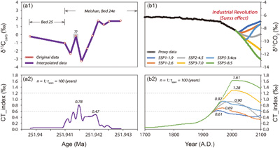 Figure 3 Comparison of δ13Ccarb and δ13CO2 across the PTr mass extinction and the Industrial Revolution period, and the calculated CTindex. (a) PTr dataset collected from bed 24e to 25, Meishan section (Burgess et al., 2014). (b) Industrial Revolution period (Rubino et al., 2013). The future δ13CO2 estimations are based on CMIP6 Scenario-MIP (Graven et al., 2020). All the original data were interpolated to a one point per year resolution; τspan = 0.0001 Ma (100 year) and n = 1 were employed to run the CTindex. |
| Figure 1 | Figure 2 | Figure 3 |
top
Introduction
The evolution of life on Earth has been punctuated by extreme environmental/climatic events, often leading to mass extinctions (Chen and Benton, 2012
Chen, Z.-Q., Benton, M.J. (2012) The timing and pattern of biotic recovery following the end-Permian mass extinction. Nature Geoscience 5, 375–383.
; Rothman, 2017Rothman, D.H. (2017) Thresholds of catastrophe in the Earth system. Science Advances 3, e1700906.
). Carbon cycle perturbations, global warming or cooling, and widespread anoxia have all played major roles in shaping the course of biotic macroevolution (Payne et al., 2020Payne, J.L, Bachan, A, Heim, N.A, Hull, P.M, Knope, M.L. (2020) The evolution of complex life and the stabilization of the Earth system. Interface Focus 10, 20190106.
). However, there is no general model that encompasses the range of scenarios documented by the geological record. For example, in terms of global δ13C records, negative (e.g., end Permian) and positive (e.g., end Ordovician) excursions have both been linked to biotic extinctions (Fan et al., 2020Fan, J.X., Shen, S.Z., Erwin, D.H., Sadler, P.M., Macleod, N., Cheng, Q.M., Hou, X.D., Yang, J., Wang, X.D., Wang, Y., Zhang, H., Chen, X., Li, G.X., Zhang, Y.C., Shi, Y.K., Yuan, D.X., Chen, Q., Zhang, L.N., Li, C., Zhao, Y.Y. (2020) A high-resolution summary of Cambrian to Early Triassic marine invertebrate biodiversity. Science 367, 272–277.
). Thus, while major biotic events were linked to intervals of environmental perturbation and ecologic disturbance, they were not universally driven by one particular environmental process. However, there are no reliable proxies for measuring the extent of carbon cycle instability and associated environmental stress through Earth history.Here, we develop a carbon cycle turbulence index (CTindex) to measure perturbations in the δ13Ccarb record (Cramer and Jarvis, 2020
Cramer, B.D., Jarvis, I. (2020) Chapter 11 - Carbon Isotope Stratigraphy. In: Gradstein, F.M., Ogg, J.G., Schmitz, M.D., Ogg, G.M. (Eds.) The Geologic Time Scale 2020. Elsevier, Amsterdam, 309–343. https://doi.org/10.1016/B978-0-12-824360-2.00011-5
) over the last 1,000 Myr. The CTindex emphasises perturbations to the carbon cycle as a metric for ecosystem instability. The rationale for using δ13Ccarb perturbation is because the δ13Ccarb record is robust and at high resolution, and short term (0.5–10 Myr) δ13Ccarb variability over the past 1,000 Myr has been suggested to record ocean-atmosphere system instability (Rothman, 2017Rothman, D.H. (2017) Thresholds of catastrophe in the Earth system. Science Advances 3, e1700906.
). The CTindex is calculated according to Equation 1:Eq. 1
To measure the degree of carbon cycle turbulence at each point (CTindex (t)), over a pre-determined duration (e.g., τspan = 0.05 Myr), we compiled all the datum points within the τspan (centred on the calculating point, t) in array F. In this case, N and μ(t) represent the number and average isotopic value of the array F, respectively, where n is a statistical control to avoid a situation where the sum of the mean deviations is zero. When n = 2, the output of the calculation, CTindex (t), is equal to the standard deviation of the array F (see sensitivity tests for parameters τspan and n in Supplementary Information). Thus, major positive and negative excursions will both result in a CTindex peak.
Phanerozoic biotic extinction rates (ERs) at the generic level were derived from a palaeobiology database (PaleoDB), and are applied to represent biodiversity changes and ecologic disturbance for comparison with CTindex values (Fig. 1). The fossil record often documents a direct link between enhanced ERs and dramatic reductions in biodiversity, or major ecologic disturbance, during mass extinctions (Alroy et al., 2008
Alroy, J., Aberhan, M., Bottjer, D., Foote, M., Fursich, F.T., Harries, P.J., Hendy, A.J.W., Holland, S.M., Lvany, L.C., Kiessling, W., Kosnik, M.A., Marshall, C.R., McGowan, A.J., Miller, A.I., Olszewski, T.D., Patzkowsky, M.E., Peters, S.E., Villier, L., Wagner, P.J., Bonuso, N., Borkow, P.S., Brenneis, B., Clapham, M.E., Fall, L.M., Ferguson, C.A., Hanson, V.L., Krug, A.Z., Layou, K.M., Leckey, E.H., Nurnberg, S., Powers, C.M., Sessa, J.A., Simpson, C., Tomasovych, A., Visaggi, C.C. (2008) Phanerozoic Trends in the Global Diversity of Marine Invertebrates. Science 321, 97–100.
). Hence, relationships between CTindex peaks and higher ER values can be employed to investigate coincidence between catastrophic environmental stress and biotic crises through Earth history. Moreover, increasing evidence suggests that we are in the midst of a “sixth mass extinction” (Barnosky et al., 2011Barnosky, A.D., Matzke, N., Tomiya, S., Wogan, G.O.U., Swartz, B., Quental, T.B., Marshall, C., McGuire, J.L., Lindsey, E., Maguire, K.C., Mersey, B., Ferrer, E.A. (2011) Has the Earth’s sixth mass extinction already arrived? Nature 471, 51–57.
; Ceballos et al., 2015Ceballos, G., Ehrlich, P.R., Barnosky, A.D., García, A., Pringle, R.M., Palmer, T.M. (2015) Accelerated modern human–induced species losses: Entering the sixth mass extinction. Science Advances 1, e1400253.
), and a pronounced negative excursion in δ13CO2 caused by greenhouse gas emissions has been recorded since the onset of the industrial revolution (Graven et al., 2020Graven, H., Keeling, R.F., Rogelj, J. (2020) Changes to Carbon Isotopes in Atmospheric CO2 Over the Industrial Era and Into the Future. Global Biogeochemical Cycles 34, e2019GB006170.
). In order to investigate the current and potential future significance of rising greenhouse gas emissions on biotic ERs, we compare the present day CTindex value to that observed during the Permian/Triassic (PTr) transition, representing the most severe mass extinction of the Phanerozoic.Figure 1 δ13Ccarb database (Cramer and Jarvis, 2020
Cramer, B.D., Jarvis, I. (2020) Chapter 11 - Carbon Isotope Stratigraphy. In: Gradstein, F.M., Ogg, J.G., Schmitz, M.D., Ogg, G.M. (Eds.) The Geologic Time Scale 2020. Elsevier, Amsterdam, 309–343. https://doi.org/10.1016/B978-0-12-824360-2.00011-5
) and calculated CTindex values across the last 1,000 Myr, combined with calculated extinction rates through the Phanerozoic (from the palaeobiology database; http://www.paleobiodb.org/; Kocsis et al., 2019Kocsis, A.T., Reddin, C.J., Alroy, J., Kiessling, W. (2019) The r package divDyn for quantifying diversity dynamics using fossil sampling data. Methods in Ecology and Evolution 10, 735–743.
).top
Results and Discussion
CTindex vs. environmental perturbations. Our reconstruction of the CTindex through time (Fig. 1; analytical methods and database details are given in the Supplementary Information) highlights that it is both the magnitude and duration of the carbon cycle perturbation that exhibits a major link to the extent of environmental and biotic change. The CTindex offers a unique measure of the intensity of δ13Ccarb fluctuations, which reflect carbon cycle perturbation and the dynamic balance between the input of carbon and its burial as carbonate and organic matter (Kump and Arthur, 1999
Kump, L.R., Arthur, M.A. (1999) Interpreting carbon-isotope excursions: carbonates and organic matter. Chemical Geology 161, 181–198.
). As such, the CTindex peaks during the late Tonian, through the Cryogenian and Ediacaran glaciations, and into the Cambrian (Fig. 1), broadly correlate with periods of environmental oxygenation (Canfield et al., 2007Canfield, D.E., Poulton, S.W., Narbonne, G.M. (2007) Late-Neoproterozoic Deep-Ocean Oxygenation and the Rise of Animal Life. Science, New Series 315, 92–95.
; Lyons et al., 2021Lyons, T.W., Diamond, C.W., Planavsky, N.J., Reinhard, C.T., Li, C. (2021) Oxygenation, Life, and the Planetary System during Earth’s Middle History: An Overview. Astrobiology 21, 906–923.
). The major variability evident in CTindex values (in both magnitude and frequency) reflects well documented instability in the extent of Earth surface oxygenation over this interval (Canfield et al., 2008Canfield, D.E., Poulton, S.W., Knoll, A.H., Narbonne, G.M., Ross, G., Goldberg, T., Strauss, H. (2008) Ferruginous Conditions Dominated Later Neoproterozoic Deep-Water Chemistry. Science 321, 949–952.
; Sahoo et al., 2016Sahoo, S.K., Planavsky, N.J., Jiang, G., Kendall, B., Owens, J.D., Wang, X., Shi, X., Anbar, A.D., Lyons, T.W. (2016) Oceanic oxygenation events in the anoxic Ediacaran ocean. Geobiology 14, 457–468.
; He et al., 2019He, T.C., Zhu, M.Y., Mills, B.J.W., Wynn, P.M., Zhuravlev, A.Y., Tostevin, R., Pogge Von Strandmann, P.A.E., Yang, A.H., Poulton, S.W., Shields, G.A. (2019) Possible links between extreme oxygen perturbations and the Cambrian radiation of animals. Nature Geoscience 12, 468–474.
; Li et al., 2020Li, Z., Cao, M., Loyd, S.J., Algeo, T.J., Zhao, H., Wang, X., Zhao, L., Chen, Z.-Q. (2020) Transient and stepwise ocean oxygenation during the late Ediacaran Shuram Excursion: Insights from carbonate δ238U of northwestern Mexico. Precambrian Research 344, 105741.
).As the Earth progressed to near modern levels of oxygenation in the Palaeozoic (Krause et al., 2018
Krause, A.J., Mills, B.J.W., Zhang, S., Planavsky, N.J., Lenton, T.M., Poulton, S.W. (2018) Stepwise oxygenation of the Paleozoic atmosphere. Nature Communications 9, 4081.
) and life continued to evolve and diversify (Lenton et al., 2016Lenton, T.M., Dahl, T.W., Daines, S.J., Mills, B.J.W., Ozaki, K., Saltzman, M.R., Porada, P. (2016) Earliest land plants created modern levels of atmospheric oxygen. PNAS 113, 9704–9709.
), the ensuing environmental stability generally resulted in lower peaks in CTindex values, with the exception of the major peak across the PTr boundary (Fig. 1). However, despite the general decrease, the CTindex trend is of sufficient resolution (see Fig. S-4) to distinguish nearly all of the major individual carbon cycle perturbations during the Phanerozoic (Fig. 1). Thus, although there are many potential controls on the δ13Ccarb record (Lenton et al., 2018Lenton, T.M., Daines, S.J. (2018) The effects of marine eukaryote evolution on phosphorus, carbon and oxygen cycling across the Proterozoic–Phanerozoic transition. Emerging Topics in Life Sciences 2, 267–278.
), the CTindex provides an integrated and robust assessment of the overall extent of environmental perturbation.Deciphering extinction rates and environmental perturbations. The CTindex trends correlate with biodiversity fluctuations, ERs and ecologic disturbance through the Neoproterozoic and Phanerozoic (Fig. 1). Several important intervals of biodiversification, including the initial evolution of the Ediacaran biota, the Cambrian explosion, the Great Ordovician Biodiversification, the Carboniferous-Permian, and the mid-Triassic and Jurassic-Cretaceous radiations (Sepkoski, 1981
Sepkoski, J.J. (1981) A factor analytic description of the Phanerozoic marine fossil record. Paleobiology 7, 36–53.
; Alroy et al., 2008Alroy, J., Aberhan, M., Bottjer, D., Foote, M., Fursich, F.T., Harries, P.J., Hendy, A.J.W., Holland, S.M., Lvany, L.C., Kiessling, W., Kosnik, M.A., Marshall, C.R., McGowan, A.J., Miller, A.I., Olszewski, T.D., Patzkowsky, M.E., Peters, S.E., Villier, L., Wagner, P.J., Bonuso, N., Borkow, P.S., Brenneis, B., Clapham, M.E., Fall, L.M., Ferguson, C.A., Hanson, V.L., Krug, A.Z., Layou, K.M., Leckey, E.H., Nurnberg, S., Powers, C.M., Sessa, J.A., Simpson, C., Tomasovych, A., Visaggi, C.C. (2008) Phanerozoic Trends in the Global Diversity of Marine Invertebrates. Science 321, 97–100.
; Erwin et al., 2011Erwin, D.H., Laflamme, M., Tweedt, S.M., Sperling, E.A., Pisani, D., Peterson, K.J. (2011) The Cambrian Conundrum: Early Divergence and Later Ecological Success in the Early History of Animals. Science 334, 1091–1097.
; Darroch et al., 2018Darroch, S.A.F., Smith, E.F., Laflamme, M., Erwin, D.H. (2018) Ediacaran Extinction and Cambrian Explosion. Trends in Ecology & Evolution 33, 653–663.
; Fan et al., 2020Fan, J.X., Shen, S.Z., Erwin, D.H., Sadler, P.M., Macleod, N., Cheng, Q.M., Hou, X.D., Yang, J., Wang, X.D., Wang, Y., Zhang, H., Chen, X., Li, G.X., Zhang, Y.C., Shi, Y.K., Yuan, D.X., Chen, Q., Zhang, L.N., Li, C., Zhao, Y.Y. (2020) A high-resolution summary of Cambrian to Early Triassic marine invertebrate biodiversity. Science 367, 272–277.
), all coincide with low CTindex values. By contrast, pronounced CTindex peaks correspond to higher ERs, as evident during mass extinctions (Fig. 1b).However, since the datum sampling densities of δ13Ccarb database and PaleoDB are clearly different, it is difficult to directly calculate the regression relationship between the CTindex and ERs. To address this, we begin by identifying significant global perturbation events during the Phanerozoic (Fig. S-4, Table S-2). These 41 events comprise the major δ13Ccarb perturbations (Rothman, 2017
Rothman, D.H. (2017) Thresholds of catastrophe in the Earth system. Science Advances 3, e1700906.
), mass extinctions (Bambach, 2006Bambach, R.K. (2006) Phanerozoic Biodiversity Mass Extinctions. Annual Review of Earth and Planetary Sciences 34, 127–155.
), and biodiversifications (Fan et al., 2020Fan, J.X., Shen, S.Z., Erwin, D.H., Sadler, P.M., Macleod, N., Cheng, Q.M., Hou, X.D., Yang, J., Wang, X.D., Wang, Y., Zhang, H., Chen, X., Li, G.X., Zhang, Y.C., Shi, Y.K., Yuan, D.X., Chen, Q., Zhang, L.N., Li, C., Zhao, Y.Y. (2020) A high-resolution summary of Cambrian to Early Triassic marine invertebrate biodiversity. Science 367, 272–277.
). While the CTindex trend reflects the degree of environmental perturbation on the timescale of individual events (Fig. S-3), consideration needs to be given to the method for calculating ER ratios. Kocsis et al. (2019)Kocsis, A.T., Reddin, C.J., Alroy, J., Kiessling, W. (2019) The r package divDyn for quantifying diversity dynamics using fossil sampling data. Methods in Ecology and Evolution 10, 735–743.
explored 12 different metrics to calculate ER values (Fig. 1b), which also consider the potential errors caused by the PaleoDB itself. For each stage, we use the maximum, minimum and ‘sqs2f3’ methods (Kocsis et al., 2019Kocsis, A.T., Reddin, C.J., Alroy, J., Kiessling, W. (2019) The r package divDyn for quantifying diversity dynamics using fossil sampling data. Methods in Ecology and Evolution 10, 735–743.
) to establish a broad range for the calculation of ER values (Fig. 2, Fig. S-5). Then, each major CTindex peak is considered responsible for the corresponding ER perturbation.Figure 2 Cross plots of the extinction rate (ER) vs. the CTindex for 41 events. (a) Blue circles represent outlier events from the Cambrian and Silurian. Red circles represent the other events from the Phanerozoic, which show a strong correlation between ER and the CTindex. (b) Logarithmic plot of the extinction rate (ER) vs. the CTindex for 41 events, with the best fit logistic regression curve of the red circles. See Table S-2 for details.
Cross plots show that the CTindex and ER values for 31 of these events are broadly positively correlated (red points; Fig. 2), with R2 = 0.835 and p < 0.001. The remaining 10 events (blue points; Fig. 2) comprise two types of outlier: (1) events with high ER and low CTindex values, occurring from 541 to 480 Ma (from the Cambrian to the first stage of the Ordovician), and (2) events with high CTindex and low ER values, occurring in Silurian. Given that the dataset for these latter two intervals is smaller than that of other periods of the Phanerozoic (Fig. S-4a), these outliers may result from the incompleteness of the PaleoDB. However, a fundamental difference in ecosystem stability for these periods, relative to the rest of the Phanerozoic, cannot be ruled out. Nevertheless, the CTindex suggests that environmental turbulence was intense during the early Cambrian (but not the middle to late Cambrian) and through the entire Silurian. While the high ER and low CTindex signal for 541–480 Ma may represent an unstable ecosystem, the high CTindex and low ER signal for the Silurian reflects a more stable ecosystem that did not suffer a major extinction.
Next, in order to explore the potential thresholds of the mass extinctions, we use a logistic curve (sigmoid curve) to fit the data (Fig. 2b), which is a widely used approach for deep time extinction studies (Roopnarine, 2006
Roopnarine, P.D. (2006) Extinction cascades and catastrophe in ancient food webs. Paleobiology 32, 1–19.
). Logistic curves represent the battle between ecosystem stability and environmental instability. Ecosystems are generally unaffected at low levels of volatility, but when the degree of volatility increases to a certain threshold, the biotic ER rapidly increases (e.g., the PTr and TJ mass extinctions).In addition to distinguishing these well studied events, the logistic curve also provides new insight into broader trends through time. Here we note that a previous study of major δ13Ccarb events suggests that the thresholds of catastrophe in the Earth system have not changed systematically over time (Rothman, 2017
Rothman, D.H. (2017) Thresholds of catastrophe in the Earth system. Science Advances 3, e1700906.
). Building on this, our data implicitly suggest that, although life has evolved into more complex forms, ecosystem tolerance to environmental turbulence has not significantly improved through time (discounting the Cambrian and Silurian; Fig. S-5c). This observation naturally leads to consideration of whether the CTindex may be used to evaluate the possible nature of Earth’s “sixth mass extinction” in the modern and future environment.Contrasting the CTindex during the PTr and from 1700 to 2100 A.D. Current high extinction rates of some taxonomic groups suggest that the Earth may be entering a “sixth mass extinction”, which may have a causal relationship with increasing greenhouse gases in the atmosphere (Barnosky et al., 2011
Barnosky, A.D., Matzke, N., Tomiya, S., Wogan, G.O.U., Swartz, B., Quental, T.B., Marshall, C., McGuire, J.L., Lindsey, E., Maguire, K.C., Mersey, B., Ferrer, E.A. (2011) Has the Earth’s sixth mass extinction already arrived? Nature 471, 51–57.
; Ceballos et al., 2015Ceballos, G., Ehrlich, P.R., Barnosky, A.D., García, A., Pringle, R.M., Palmer, T.M. (2015) Accelerated modern human–induced species losses: Entering the sixth mass extinction. Science Advances 1, e1400253.
). However, there is still a widely recognised “last kilometre gap” between the fossil record and the modern bio-record and their extinction rates, for the following reasons: (1) most modern data focus on terrestrial vertebrates (e.g., mammals and birds), whereas the fossil record dominantly reflects marine invertebrates (e.g., brachiopods, gastropods and bivalves) (Kocsis et al., 2019Kocsis, A.T., Reddin, C.J., Alroy, J., Kiessling, W. (2019) The r package divDyn for quantifying diversity dynamics using fossil sampling data. Methods in Ecology and Evolution 10, 735–743.
), and (2) there are different time spans when considering a particular extinction. Specifically, the “Big Five” Phanerozoic mass extinctions are only constrained across a broad time resolution of millions of years, so a comparison with modern events occurring on a timescale of a hundred to a thousand years is not straightforward, and (3) there is uncertainty in the near future. For example, calculation of ERs for modern species is hampered since it remains unknown whether “critically endangered species” will actually go extinct (Barnosky et al., 2011Barnosky, A.D., Matzke, N., Tomiya, S., Wogan, G.O.U., Swartz, B., Quental, T.B., Marshall, C., McGuire, J.L., Lindsey, E., Maguire, K.C., Mersey, B., Ferrer, E.A. (2011) Has the Earth’s sixth mass extinction already arrived? Nature 471, 51–57.
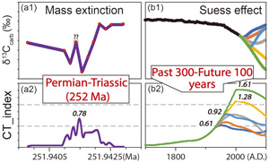
). (4) Other unknowns, including continental configuration, pre-existing climate state, and the extant biota at the time of CTindex perturbation might also affect how the ER responds.To address these issues, we note that if the core hypothesis of the CTindex stands, then the sixth mass extinction should be accompanied by a distinct CTindex peak. We thus reconstruct CTindex values from 1700 to 2100 A.D., representing the time period prior to, and after, the industrial revolution, and we contrast this with the PTr transition at ∼252 Ma, representing the most severe mass extinction of the Phanerozoic. We used δ13CO2 curves from ice core to reconstruct the modern CTindex trend due to its complete and robust record over the last several centuries, in addition to the availability of modelled near future values (Rubino et al., 2013
Rubino, M., Etheridge, D.M., Trudinger, C.M., Allison, C.E., Battle, M.O., Langenfelds, R.L., Steele, L.P., Curran, M., Bender, M., White, J.W.C., Jenk, T.M., Blunier, T., Francey, R.T. (2013) A revised 1000 year atmospheric δ13C‐CO2 record from Law Dome and South Pole, Antarctica. Journal of Geophysical Research: Atmospheres 118, 8482–8499.
; Graven et al., 2020Graven, H., Keeling, R.F., Rogelj, J. (2020) Changes to Carbon Isotopes in Atmospheric CO2 Over the Industrial Era and Into the Future. Global Biogeochemical Cycles 34, e2019GB006170.
). However, we note that other carbon hosts, including surface ocean dissolved inorganic carbon, coral samples, and CH4 in Antarctica ice core also sensitively record significant CTindex peaks (Fig. S-7). This approach is reinforced by an observed strong similarity in the CTindex output when calculated using the δ13CO2 and δ13C coral records (Fig. S-7). To further enhance the reliability of our comparison, we focus on a very short interval during the PTr transition, between Bed 24e to Bed 25 in the Meishan GSSP section, which documents the extinction level itself (Burgess et al., 2014Burgess, S.D., Bowring, S., Shen, S. (2014) High-precision timeline for Earth’s most severe extinction. PNAS 111, 3316–3321.
). This interval has 11 original δ13Ccarb datum points across an estimated interval of ∼3,000 years. Hence, we calculate the CTindex for both the PTr and the industrial revolution period using the same parameters (n = 1; τspan = 100 years), and the datasets were pre-normalised to a datum density of one point per year.The relative size of the CTindex peaks calculated under the same conditions for the two time intervals is of practical comparative significance (Fig. 3). The CTindex peak during the PTr ranges from 0.47 to 0.78, whilst the CTindex peak of the industrial revolution period ranges from 0.61 to 1.61, with the latter reflecting the predicted range for the δ13CO2 trend into the near future. If fossil fuel emissions peak at the present level and are at a low level through the next century, it has been suggested (Graven et al., 2020
Graven, H., Keeling, R.F., Rogelj, J. (2020) Changes to Carbon Isotopes in Atmospheric CO2 Over the Industrial Era and Into the Future. Global Biogeochemical Cycles 34, e2019GB006170.
) that δ13CO2 may recover from −8.8 ‰ to 7.0 ‰, which leads to a moderate CTindex peak (line SSP1-1.9; Fig. 3). However, in other scenarios without such effective limits on fossil fuel emissions, δ13CO2 will likely continue to decrease through the next century (line SSP8.5), causing a dramatic peak in the CTindex that may be even greater than the PTr CTindex peak (Fig. 3). While the current extinction of species is driven by biodiversity loss that is only partly associated with fossil fuel driven climate change, the empirical relationship between ecosystem stability and biotic ERs implies that, if fossil fuel emissions are not significantly decreased, Earth’s “sixth mass extinction” has the potential to be severe.Figure 3 Comparison of δ13Ccarb and δ13CO2 across the PTr mass extinction and the Industrial Revolution period, and the calculated CTindex. (a) PTr dataset collected from bed 24e to 25, Meishan section (Burgess et al., 2014
Burgess, S.D., Bowring, S., Shen, S. (2014) High-precision timeline for Earth’s most severe extinction. PNAS 111, 3316–3321.
). (b) Industrial Revolution period (Rubino et al., 2013Rubino, M., Etheridge, D.M., Trudinger, C.M., Allison, C.E., Battle, M.O., Langenfelds, R.L., Steele, L.P., Curran, M., Bender, M., White, J.W.C., Jenk, T.M., Blunier, T., Francey, R.T. (2013) A revised 1000 year atmospheric δ13C‐CO2 record from Law Dome and South Pole, Antarctica. Journal of Geophysical Research: Atmospheres 118, 8482–8499.
). The future δ13CO2 estimations are based on CMIP6 Scenario-MIP (Graven et al., 2020Graven, H., Keeling, R.F., Rogelj, J. (2020) Changes to Carbon Isotopes in Atmospheric CO2 Over the Industrial Era and Into the Future. Global Biogeochemical Cycles 34, e2019GB006170.
). All the original data were interpolated to a one point per year resolution; τspan = 0.0001 Ma (100 year) and n = 1 were employed to run the CTindex.top
Acknowledgements
The contributors to the PaleoDB database and Geologic Time Scale are thanked for their provision of taxonomic and carbon isotope data for the database. We are grateful to Gavin Foster and two anonymous reviewers for their comments, which greatly improved this manuscript. This study was supported by five NSFC grants (41821001, 41930322, 41977264, 42073002, 92055212), and by 111 Project of China (BP0820004). ZL is funded by the Fundamental Research Funds for National Universities, China University of Geosciences (Wuhan).
Editor: Gavin Foster
top
References
Alroy, J., Aberhan, M., Bottjer, D., Foote, M., Fursich, F.T., Harries, P.J., Hendy, A.J.W., Holland, S.M., Lvany, L.C., Kiessling, W., Kosnik, M.A., Marshall, C.R., McGowan, A.J., Miller, A.I., Olszewski, T.D., Patzkowsky, M.E., Peters, S.E., Villier, L., Wagner, P.J., Bonuso, N., Borkow, P.S., Brenneis, B., Clapham, M.E., Fall, L.M., Ferguson, C.A., Hanson, V.L., Krug, A.Z., Layou, K.M., Leckey, E.H., Nurnberg, S., Powers, C.M., Sessa, J.A., Simpson, C., Tomasovych, A., Visaggi, C.C. (2008) Phanerozoic Trends in the Global Diversity of Marine Invertebrates. Science 321, 97–100. https://doi.org/10.1126/science.1156963
 Show in context
 The fossil record often documents a direct link between enhanced ERs and dramatic reductions in biodiversity, or major ecologic disturbance, during mass extinctions (Alroy et al., 2008).
View in article
Several important intervals of biodiversification, including the initial evolution of the Ediacaran biota, the Cambrian explosion, the Great Ordovician Biodiversification, the Carboniferous-Permian, and the mid-Triassic and Jurassic-Cretaceous radiations (Sepkoski, 1981; Alroy et al., 2008; Erwin et al., 2011; Darroch et al., 2018; Fan et al., 2020), all coincide with low CTindex values.
View in article
Bambach, R.K. (2006) Phanerozoic Biodiversity Mass Extinctions. Annual Review of Earth and Planetary Sciences 34, 127–155. https://doi.org/10.1146/annurev.earth.33.092203.122654
Show in context These 41 events comprise the major δ13Ccarb perturbations (Rothman, 2017), mass extinctions (Bambach, 2006), and biodiversifications (Fan et al., 2020).
View in article
Barnosky, A.D., Matzke, N., Tomiya, S., Wogan, G.O.U., Swartz, B., Quental, T.B., Marshall, C., McGuire, J.L., Lindsey, E., Maguire, K.C., Mersey, B., Ferrer, E.A. (2011) Has the Earth’s sixth mass extinction already arrived? Nature 471, 51–57. https://doi.org/10.1038/nature09678
Show in context Moreover, increasing evidence suggests that we are in the midst of a “sixth mass extinction” (Barnosky et al., 2011; Ceballos et al., 2015), and a pronounced negative excursion in δ13CO2 caused by greenhouse gas emissions has been recorded since the onset of the industrial revolution (Graven et al., 2020).
View in article
For example, calculation of ERs for modern species is hampered since it remains unknown whether “critically endangered species” will actually go extinct (Barnosky et al., 2011).
View in article
Current high extinction rates of some taxonomic groups suggest that the Earth may be entering a “sixth mass extinction”, which may have a causal relationship with increasing greenhouse gases in the atmosphere (Barnosky et al., 2011; Ceballos et al., 2015).
View in article
Burgess, S.D., Bowring, S., Shen, S. (2014) High-precision timeline for Earth’s most severe extinction. PNAS 111, 3316–3321. https://doi.org/10.1073/pnas.1317692111
Show in context To further enhance the reliability of our comparison, we focus on a very short interval during the PTr transition, between Bed 24e to Bed 25 in the Meishan GSSP section, which documents the extinction level itself (Burgess et al., 2014).
View in article
(a) PTr dataset collected from bed 24e to 25, Meishan section (Burgess et al., 2014).
View in article
Canfield, D.E., Poulton, S.W., Narbonne, G.M. (2007) Late-Neoproterozoic Deep-Ocean Oxygenation and the Rise of Animal Life. Science, New Series 315, 92–95. https://doi.org/10.1126/science.1135013
Show in context As such, the CTindex peaks during the late Tonian, through the Cryogenian and Ediacaran glaciations, and into the Cambrian (Fig. 1), broadly correlate with periods of environmental oxygenation (Canfield et al., 2007; Lyons et al., 2021).
View in article
Canfield, D.E., Poulton, S.W., Knoll, A.H., Narbonne, G.M., Ross, G., Goldberg, T., Strauss, H. (2008) Ferruginous Conditions Dominated Later Neoproterozoic Deep-Water Chemistry. Science 321, 949–952. https://doi.org/10.1126/science.1154499
Show in context The major variability evident in CTindex values (in both magnitude and frequency) reflects well documented instability in the extent of Earth surface oxygenation over this interval (Canfield et al., 2008; Sahoo et al., 2016; He et al., 2019; Li et al., 2020).
View in article
Ceballos, G., Ehrlich, P.R., Barnosky, A.D., García, A., Pringle, R.M., Palmer, T.M. (2015) Accelerated modern human–induced species losses: Entering the sixth mass extinction. Science Advances 1, e1400253. https://doi.org/10.1126/sciadv.1400253
Show in context Moreover, increasing evidence suggests that we are in the midst of a “sixth mass extinction” (Barnosky et al., 2011; Ceballos et al., 2015), and a pronounced negative excursion in δ13CO2 caused by greenhouse gas emissions has been recorded since the onset of the industrial revolution (Graven et al., 2020).
View in article
Current high extinction rates of some taxonomic groups suggest that the Earth may be entering a “sixth mass extinction”, which may have a causal relationship with increasing greenhouse gases in the atmosphere (Barnosky et al., 2011; Ceballos et al., 2015).
View in article
Chen, Z.-Q., Benton, M.J. (2012) The timing and pattern of biotic recovery following the end-Permian mass extinction. Nature Geoscience 5, 375–383. https://doi.org/10.1038/ngeo1475
Show in context The evolution of life on Earth has been punctuated by extreme environmental/climatic events, often leading to mass extinctions (Chen and Benton, 2012; Rothman, 2017).
View in article
Cramer, B.D., Jarvis, I. (2020) Chapter 11 - Carbon Isotope Stratigraphy. In: Gradstein, F.M., Ogg, J.G., Schmitz, M.D., Ogg, G.M. (Eds.) The Geologic Time Scale 2020. Elsevier, Amsterdam, 309–343. https://doi.org/10.1016/B978-0-12-824360-2.00011-5
Show in context Here, we develop a carbon cycle turbulence index (CTindex) to measure perturbations in the δ13Ccarb record (Cramer and Jarvis, 2020) over the last 1,000 Myr.
View in article
δ13Ccarb database (Cramer and Jarvis, 2020) and calculated CTindex values across the last 1,000 Myr, combined with calculated extinction rates through the Phanerozoic (from the palaeobiology database; http://www.paleobiodb.org/; Kocsis et al., 2019).
View in article
Darroch, S.A.F., Smith, E.F., Laflamme, M., Erwin, D.H. (2018) Ediacaran Extinction and Cambrian Explosion. Trends in Ecology & Evolution 33, 653–663. https://doi.org/10.1016/j.tree.2018.06.003
Show in context Several important intervals of biodiversification, including the initial evolution of the Ediacaran biota, the Cambrian explosion, the Great Ordovician Biodiversification, the Carboniferous-Permian, and the mid-Triassic and Jurassic-Cretaceous radiations (Sepkoski, 1981; Alroy et al., 2008; Erwin et al., 2011; Darroch et al., 2018; Fan et al., 2020), all coincide with low CTindex values.
View in article
Erwin, D.H., Laflamme, M., Tweedt, S.M., Sperling, E.A., Pisani, D., Peterson, K.J. (2011) The Cambrian Conundrum: Early Divergence and Later Ecological Success in the Early History of Animals. Science 334, 1091–1097. https://doi.org/10.1126/science.1206375
Show in context Several important intervals of biodiversification, including the initial evolution of the Ediacaran biota, the Cambrian explosion, the Great Ordovician Biodiversification, the Carboniferous-Permian, and the mid-Triassic and Jurassic-Cretaceous radiations (Sepkoski, 1981; Alroy et al., 2008; Erwin et al., 2011; Darroch et al., 2018; Fan et al., 2020), all coincide with low CTindex values.
View in article
Fan, J.X., Shen, S.Z., Erwin, D.H., Sadler, P.M., Macleod, N., Cheng, Q.M., Hou, X.D., Yang, J., Wang, X.D., Wang, Y., Zhang, H., Chen, X., Li, G.X., Zhang, Y.C., Shi, Y.K., Yuan, D.X., Chen, Q., Zhang, L.N., Li, C., Zhao, Y.Y. (2020) A high-resolution summary of Cambrian to Early Triassic marine invertebrate biodiversity. Science 367, 272–277. https://doi.org/10.1126/science.aax4953
Show in context For example, in terms of global δ13C records, negative (e.g., end Permian) and positive (e.g., end Ordovician) excursions have both been linked to biotic extinctions (Fan et al., 2020).
View in article
These 41 events comprise the major δ13Ccarb perturbations (Rothman, 2017), mass extinctions (Bambach, 2006), and biodiversifications (Fan et al., 2020).
View in article
Several important intervals of biodiversification, including the initial evolution of the Ediacaran biota, the Cambrian explosion, the Great Ordovician Biodiversification, the Carboniferous-Permian, and the mid-Triassic and Jurassic-Cretaceous radiations (Sepkoski, 1981; Alroy et al., 2008; Erwin et al., 2011; Darroch et al., 2018; Fan et al., 2020), all coincide with low CTindex values.
View in article
Graven, H., Keeling, R.F., Rogelj, J. (2020) Changes to Carbon Isotopes in Atmospheric CO2 Over the Industrial Era and Into the Future. Global Biogeochemical Cycles 34, e2019GB006170. https://doi.org/10.1029/2019GB006170
Show in context We used δ13CO2 curves from ice core to reconstruct the modern CTindex trend due to its complete and robust record over the last several centuries, in addition to the availability of modelled near future values (Rubino et al., 2013; Graven et al., 2020).
View in article
If fossil fuel emissions peak at the present level and are at a low level through the next century, it has been suggested (Graven et al., 2020) that δ13CO2 may recover from −8.8 ‰ to 7.0 ‰, which leads to a moderate CTindex peak (line SSP1-1.9; Fig. 3).
View in article
The future δ13CO2 estimations are based on CMIP6 Scenario-MIP (Graven et al., 2020).
View in article
Moreover, increasing evidence suggests that we are in the midst of a “sixth mass extinction” (Barnosky et al., 2011; Ceballos et al., 2015), and a pronounced negative excursion in δ13CO2 caused by greenhouse gas emissions has been recorded since the onset of the industrial revolution (Graven et al., 2020).
View in article
He, T.C., Zhu, M.Y., Mills, B.J.W., Wynn, P.M., Zhuravlev, A.Y., Tostevin, R., Pogge Von Strandmann, P.A.E., Yang, A.H., Poulton, S.W., Shields, G.A. (2019) Possible links between extreme oxygen perturbations and the Cambrian radiation of animals. Nature Geoscience 12, 468–474. https://doi.org/10.1038/s41561-019-0357-z
Show in context The major variability evident in CTindex values (in both magnitude and frequency) reflects well documented instability in the extent of Earth surface oxygenation over this interval (Canfield et al., 2008; Sahoo et al., 2016; He et al., 2019; Li et al., 2020).
View in article
Kocsis, A.T., Reddin, C.J., Alroy, J., Kiessling, W. (2019) The r package divDyn for quantifying diversity dynamics using fossil sampling data. Methods in Ecology and Evolution 10, 735–743. https://doi.org/10.1111/2041-210X.13161
Show in context Kocsis et al. (2019) explored 12 different metrics to calculate ER values (Fig. 1b), which also consider the potential errors caused by the PaleoDB itself.
View in article
For each stage, we use the maximum, minimum and ‘sqs2f3’ methods (Kocsis et al., 2019) to establish a broad range for the calculation of ER values (Fig. 2, Fig. S-5).
View in article
However, there is still a widely recognised “last kilometre gap” between the fossil record and the modern bio-record and their extinction rates, for the following reasons: (1) most modern data focus on terrestrial vertebrates (e.g., mammals and birds), whereas the fossil record dominantly reflects marine invertebrates (e.g., brachiopods, gastropods and bivalves) (Kocsis et al., 2019), and (2) there are different time spans when considering a particular extinction.
View in article
δ13Ccarb database (Cramer and Jarvis, 2020) and calculated CTindex values across the last 1,000 Myr, combined with calculated extinction rates through the Phanerozoic (from the palaeobiology database; http://www.paleobiodb.org/; Kocsis et al., 2019).
View in article
Krause, A.J., Mills, B.J.W., Zhang, S., Planavsky, N.J., Lenton, T.M., Poulton, S.W. (2018) Stepwise oxygenation of the Paleozoic atmosphere. Nature Communications 9, 4081. https://doi.org/10.1038/s41467-018-06383-y
Show in context As the Earth progressed to near modern levels of oxygenation in the Palaeozoic (Krause et al., 2018) and life continued to evolve and diversify (Lenton et al., 2016), the ensuing environmental stability generally resulted in lower peaks in CTindex values, with the exception of the major peak across the PTr boundary (Fig. 1).
View in article
Kump, L.R., Arthur, M.A. (1999) Interpreting carbon-isotope excursions: carbonates and organic matter. Chemical Geology 161, 181–198. https://doi.org/10.1016/S0009-2541(99)00086-8
Show in context The CTindex offers a unique measure of the intensity of δ13Ccarb fluctuations, which reflect carbon cycle perturbation and the dynamic balance between the input of carbon and its burial as carbonate and organic matter (Kump and Arthur, 1999).
View in article
Lenton, T.M., Daines, S.J. (2018) The effects of marine eukaryote evolution on phosphorus, carbon and oxygen cycling across the Proterozoic–Phanerozoic transition. Emerging Topics in Life Sciences 2, 267–278. https://doi.org/10.1042/ETLS20170156
Show in context Thus, although there are many potential controls on the δ13Ccarb record (Lenton et al., 2018), the CTindex provides an integrated and robust assessment of the overall extent of environmental perturbation.
View in article
Lenton, T.M., Dahl, T.W., Daines, S.J., Mills, B.J.W., Ozaki, K., Saltzman, M.R., Porada, P. (2016) Earliest land plants created modern levels of atmospheric oxygen. PNAS 113, 9704–9709. https://doi.org/10.1073/pnas.1604787113
Show in context As the Earth progressed to near modern levels of oxygenation in the Palaeozoic (Krause et al., 2018) and life continued to evolve and diversify (Lenton et al., 2016), the ensuing environmental stability generally resulted in lower peaks in CTindex values, with the exception of the major peak across the PTr boundary (Fig. 1).
View in article
Li, Z., Cao, M., Loyd, S.J., Algeo, T.J., Zhao, H., Wang, X., Zhao, L., Chen, Z.-Q. (2020) Transient and stepwise ocean oxygenation during the late Ediacaran Shuram Excursion: Insights from carbonate δ238U of northwestern Mexico. Precambrian Research 344, 105741. https://doi.org/10.1016/j.precamres.2020.105741
Show in context The major variability evident in CTindex values (in both magnitude and frequency) reflects well documented instability in the extent of Earth surface oxygenation over this interval (Canfield et al., 2008; Sahoo et al., 2016; He et al., 2019; Li et al., 2020).
View in article
Lyons, T.W., Diamond, C.W., Planavsky, N.J., Reinhard, C.T., Li, C. (2021) Oxygenation, Life, and the Planetary System during Earth’s Middle History: An Overview. Astrobiology 21, 906–923. https://doi.org/10.1089/ast.2020.2418
Show in context As such, the CTindex peaks during the late Tonian, through the Cryogenian and Ediacaran glaciations, and into the Cambrian (Fig. 1), broadly correlate with periods of environmental oxygenation (Canfield et al., 2007; Lyons et al., 2021).
View in article
Payne, J.L, Bachan, A, Heim, N.A, Hull, P.M, Knope, M.L. (2020) The evolution of complex life and the stabilization of the Earth system. Interface Focus 10, 20190106. https://doi.org/10.1098/rsfs.2019.0106
Show in context Carbon cycle perturbations, global warming or cooling, and widespread anoxia have all played major roles in shaping the course of biotic macroevolution (Payne et al., 2020).
View in article
Roopnarine, P.D. (2006) Extinction cascades and catastrophe in ancient food webs. Paleobiology 32, 1–19. https://doi.org/10.1666/05008.1
Show in context Next, in order to explore the potential thresholds of the mass extinctions, we use a logistic curve (sigmoid curve) to fit the data (Fig. 2b), which is a widely used approach for deep time extinction studies (Roopnarine, 2006).
View in article
Rothman, D.H. (2017) Thresholds of catastrophe in the Earth system. Science Advances 3, e1700906. https://doi.org/10.1126/sciadv.1700906
Show in context The rationale for using δ13Ccarb perturbation is because the δ13Ccarb record is robust and at high resolution, and short term (0.5–10 Myr) δ13Ccarb variability over the past 1,000 Myr has been suggested to record ocean-atmosphere system instability (Rothman, 2017).
View in article
These 41 events comprise the major δ13Ccarb perturbations (Rothman, 2017), mass extinctions (Bambach, 2006), and biodiversifications (Fan et al., 2020).
View in article
Here we note that a previous study of major δ13Ccarb events suggests that the thresholds of catastrophe in the Earth system have not changed systematically over time (Rothman, 2017).
View in article
The evolution of life on Earth has been punctuated by extreme environmental/climatic events, often leading to mass extinctions (Chen and Benton, 2012; Rothman, 2017).
View in article
Rubino, M., Etheridge, D.M., Trudinger, C.M., Allison, C.E., Battle, M.O., Langenfelds, R.L., Steele, L.P., Curran, M., Bender, M., White, J.W.C., Jenk, T.M., Blunier, T., Francey, R.T. (2013) A revised 1000 year atmospheric δ13C‐CO2 record from Law Dome and South Pole, Antarctica. Journal of Geophysical Research: Atmospheres 118, 8482–8499. https://doi.org/10.1002/jgrd.50668
Show in context (b) Industrial Revolution period (Rubino et al., 2013).
View in article
We used δ13CO2 curves from ice core to reconstruct the modern CTindex trend due to its complete and robust record over the last several centuries, in addition to the availability of modelled near future values (Rubino et al., 2013; Graven et al., 2020).
View in article
Sahoo, S.K., Planavsky, N.J., Jiang, G., Kendall, B., Owens, J.D., Wang, X., Shi, X., Anbar, A.D., Lyons, T.W. (2016) Oceanic oxygenation events in the anoxic Ediacaran ocean. Geobiology 14, 457–468. https://doi.org/10.1111/gbi.12182
Show in context The major variability evident in CTindex values (in both magnitude and frequency) reflects well documented instability in the extent of Earth surface oxygenation over this interval (Canfield et al., 2008; Sahoo et al., 2016; He et al., 2019; Li et al., 2020).
View in article
Sepkoski, J.J. (1981) A factor analytic description of the Phanerozoic marine fossil record. Paleobiology 7, 36–53. https://doi.org/10.1017/S0094837300003778
Show in context Several important intervals of biodiversification, including the initial evolution of the Ediacaran biota, the Cambrian explosion, the Great Ordovician Biodiversification, the Carboniferous-Permian, and the mid-Triassic and Jurassic-Cretaceous radiations (Sepkoski, 1981; Alroy et al., 2008; Erwin et al., 2011; Darroch et al., 2018; Fan et al., 2020), all coincide with low CTindex values.
View in article
top
Supplementary Information
The Supplementary Information includes:
- The Geochemical and Paleobiology Databases
- Analytical Approaches and Statistical Analysis
- Datum Density vs. Bias
- Comparison of Carbon Cycle Perturbations and CTindex Values between the Permian-Triassic Mass Extinction and the Industrial Revolution Period of the Anthropocene
- Tables S-1 and S-2
- Figures S-1 to S-8
- Supplementary Information References
Download the Supplementary Information (PDF).
Figures
Figure 1 δ13Ccarb database (Cramer and Jarvis, 2020
Cramer, B.D., Jarvis, I. (2020) Chapter 11 - Carbon Isotope Stratigraphy. In: Gradstein, F.M., Ogg, J.G., Schmitz, M.D., Ogg, G.M. (Eds.) The Geologic Time Scale 2020. Elsevier, Amsterdam, 309–343. https://doi.org/10.1016/B978-0-12-824360-2.00011-5
) and calculated CTindex values across the last 1,000 Myr, combined with calculated extinction rates through the Phanerozoic (from the palaeobiology database; http://www.paleobiodb.org/; Kocsis et al., 2019Kocsis, A.T., Reddin, C.J., Alroy, J., Kiessling, W. (2019) The r package divDyn for quantifying diversity dynamics using fossil sampling data. Methods in Ecology and Evolution 10, 735–743.
).
Figure 2 Cross plots of the extinction rate (ER) vs. the CTindex for 41 events. (a) Blue circles represent outlier events from the Cambrian and Silurian. Red circles represent the other events from the Phanerozoic, which show a strong correlation between ER and the CTindex. (b) Logarithmic plot of the extinction rate (ER) vs. the CTindex for 41 events, with the best fit logistic regression curve of the red circles. See Table S-2 for details.
Figure 3 Comparison of δ13Ccarb and δ13CO2 across the PTr mass extinction and the Industrial Revolution period, and the calculated CTindex. (a) PTr dataset collected from bed 24e to 25, Meishan section (Burgess et al., 2014
Burgess, S.D., Bowring, S., Shen, S. (2014) High-precision timeline for Earth’s most severe extinction. PNAS 111, 3316–3321.
). (b) Industrial Revolution period (Rubino et al., 2013Rubino, M., Etheridge, D.M., Trudinger, C.M., Allison, C.E., Battle, M.O., Langenfelds, R.L., Steele, L.P., Curran, M., Bender, M., White, J.W.C., Jenk, T.M., Blunier, T., Francey, R.T. (2013) A revised 1000 year atmospheric δ13C‐CO2 record from Law Dome and South Pole, Antarctica. Journal of Geophysical Research: Atmospheres 118, 8482–8499.
). The future δ13CO2 estimations are based on CMIP6 Scenario-MIP (Graven et al., 2020Graven, H., Keeling, R.F., Rogelj, J. (2020) Changes to Carbon Isotopes in Atmospheric CO2 Over the Industrial Era and Into the Future. Global Biogeochemical Cycles 34, e2019GB006170.
). All the original data were interpolated to a one point per year resolution; τspan = 0.0001 Ma (100 year) and n = 1 were employed to run the CTindex.