




Ocean mixing timescale through time and implications for the origin of iron formations
Affiliations | Corresponding Author | Cite as | Funding information
Published by the European Association of Geochemistry
under Creative Commons License CC BY-NC-ND 4.0
Keywords: ocean mixing timescale, neodymium isotope, banded iron formation, Precambrian oceans, paleoceanography, isotope geochemistry


- Share this article


-
Article views:3,939Cumulative count of HTML views and PDF downloads.
- Download Citation
- Rights & Permissions

top
Abstract

Figures and Tables
 Figure 1 Sensitivity of the ocean mixing timescale to Earth’s day length, tidal dissipation, surface pressure, and continental configuration. Dashed lines are data constrained model estimates of present day ventilation ages from DeVries and Primeau (2011). Symbols with black outline indicate present day baseline ages in (a), (b), (d) and ozone-less baseline ages in (c). AP: aquaplanet; LS: low latitude supercontinent; HS: high latitude supercontinents. |  Figure 2 Variation in mean benthic (a) and maximum global (b) ocean mixing timescales through time. Squares and triangles correspond to historical experiments with surface pressure of 1 bar and 2 bar, respectively. Continental configuration is represented by blue (aquaplanet), yellow (low latitude supercontinent), red (high latitude supercontinents), and green (Pangaea) symbols. The black diamond at 0 Gyr is our present day baseline experiment, while black diamonds for the historical periods give the mean values of all experiments in the respective period. The asterisk at 0.5 Gyr is modelled Phanerozoic mean benthic ventilation age from Pohl et al. (2022), and the pentagrams at 0 Gyr are data constrained model estimates of present day ventilation ages from DeVries and Primeau (2011). | 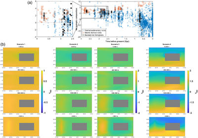 Figure 3 (a) Temporal evolution of ɛNd of Precambrian BIFs (black circles; Hu et al., 2020; Haugaard et al., 2016), depleted mantle-derived basalts (orange squares; Vervoort and Blichert-Toft, 1999) and detrital sedimentary rocks (blue triangles; Garçon, 2021). Archean Superior-type BIFs are represented by black filled circles in the zoom-in view. (b) Modelled seawater ɛNd averaged over various column depths in the Archean ocean with mean benthic ventilation age of 0.33 kyr. The four scenarios are detailed in the main text and Supplementary Information. | 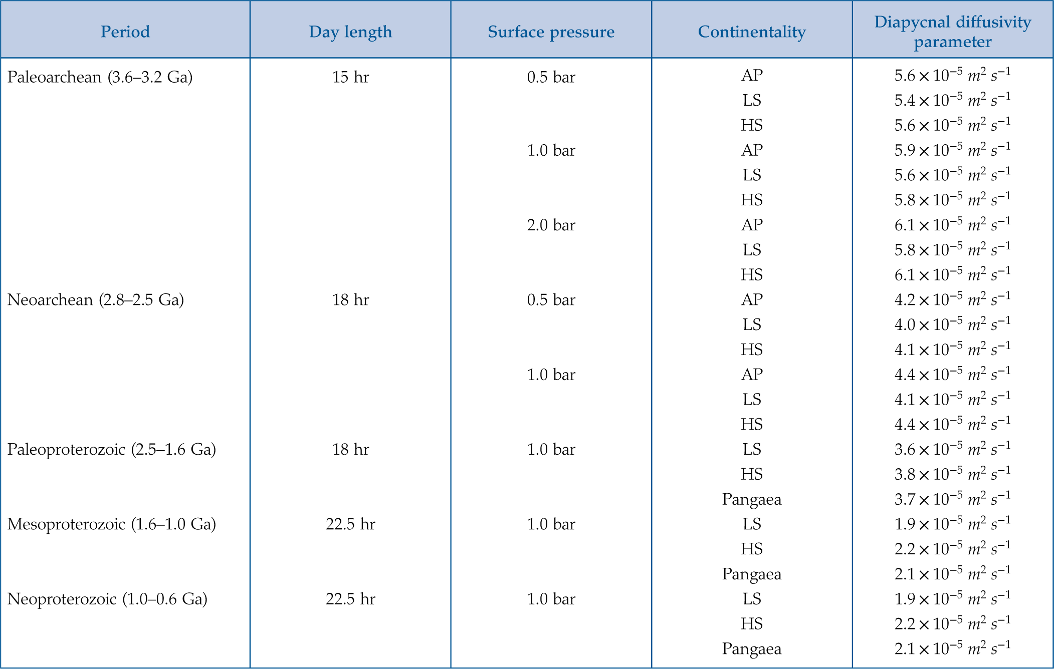 Table 1 Model setup of historical experiments. AP: aquaplanet; LS: low latitude supercontinent; HS: high latitude supercontinents. |
| Figure 1 | Figure 2 | Figure 3 | Table 1 |
top
Introduction
Ocean mixing is a key process in marine biogeochemistry, as it shapes the distribution of nutrients essential to life in the surface ocean (Meyer et al., 2016
Meyer, K.M., Ridgwell, A., Payne, J.L. (2016) The influence of the biological pump on ocean chemistry: implications for long-term trends in marine redox chemistry, the global carbon cycle, and marine animal ecosystems. Geobiology 14, 207–219. https://doi.org/10.1111/GBI.12176
) and influences the distribution of geochemical tracers in seafloor sediments that are commonly used to reconstruct ancient surface conditions (Algeo and Lyons, 2006Algeo, T.J., Lyons, T.W. (2006) Mo–total organic carbon covariation in present-day anoxic marine environments: Implications for analysis of paleoredox and paleohydrographic conditions. Paleoceanography 21, PA1016. https://doi.org/10.1029/2004PA001112
). The overall ocean mixing timescale reflects the integrated effects of both vertical and horizontal mixing processes, and the present day ocean mixing timescale is about 1 kyr (Broecker and Peng, 1982Broecker, W.S., Peng, T.H. (1982) Tracers in the Sea (vol. 690). Palisades, New York: Lamont-Doherty Geological Observatory, Columbia University. https://doi.org/10.1017/S0033822200005221
; Matsumoto, 2007Matsumoto, K. (2007) Radiocarbon‐based circulation age of the world oceans. Journal of Geophysical Research: Oceans 112, C09004. https://doi.org/10.1029/2007JC004095
). Consequently, geochemical species with residence times that are much longer than 1 kyr are generally well mixed in seawater and can thus be considered as reliable tracers of global conditions. Changes in the abundance and/or isotopic composition of these species in marine sedimentary records are often interpreted as reflecting a different balance of sources and sinks resulting from environmental changes. Other species with oceanic residence times on the order of 1 kyr or less such as neodymium (Nd), have heterogeneous isotopic compositions in modern seawater that can be used to trace mixing between different ocean basins. A very different dynamic was advocated for the Nd cycle in the Archean, with important implications for our understanding of Superior-type BIFs deposited on passive continental margins far from volcanic sources (Gross, 1972Gross, G.A. (1972) Primary features in cherty iron-formations. Sedimentary Geology 7, 241–261. https://doi.org/10.1016/0037-0738(72)90024-3
). Early studies made the case that iron in those BIFs could have come from continental weathering (James, 1954James, H.L. (1954) Sedimentary facies of iron-formation. Economic Geology 49, 235–293. https://doi.org/10.2113/gsecongeo.49.3.235
) but the present preferred hypothesis is that fluids from deep sea hydrothermal vents enriched deep ocean waters in iron, which were upwelled to continental margins where their oxidation led to BIF deposition (Derry and Jacobsen, 1988Derry, L.A., Jacobsen, S.B. (1988) The Nd and Sr isotopic evolution of Proterozoic seawater. Geophysical Research Letters 15, 397–400. https://doi.org/10.1029/GL015i004p00397
). An important argument for a hydrothermal origin of iron in Archean BIFs is the finding of positive 𝜀Nd signatures in some. We however now understand that much of the flux of Nd in the modern oceans comes from benthic sediments (95 % of all sources) (Du et al., 2020Du, J., Haley, B.A., Mix, A.C. (2020) Evolution of the Global Overturning Circulation since the Last Glacial Maximum based on marine authigenic neodymium isotopes. Quaternary Science Reviews 241, 106396. https://doi.org/10.1016/j.quascirev.2020.106396
), begging the question of whether ocean mixing would have overprinted the hydrothermal signature during transit to the continental shelf.In interpreting the chemical and isotopic compositions of sedimentary archives, it is widely assumed that the ocean mixing timescale has been similar throughout Earth’s history. However, the drivers for ocean mixing like winds, tides, or density differences, are influenced by factors like day length, surface pressure, and continental configuration that have changed through Earth’s history. For example, ocean mixing might have slowed due to shorter Archean day length (Bartlett and Stevenson, 2016
Bartlett, B.C., Stevenson, D.J. (2016) Analysis of a Precambrian resonance‐stabilized day length. Geophysical Research Letters 43, 5716–5724. https://doi.org/10.1002/2016GL068912
) by altering wind driven ocean circulation (Olson et al., 2020Olson, S.L., Jansen, M., Abbot, D.S. (2020) Oceanographic Considerations for Exoplanet Life Detection. The Astrophysical Journal 895, 19. https://doi.org/10.3847/1538-4357/ab88c9
), or due to less land exposure on early Earth (Bindeman et al., 2018Bindeman, I.N., Zakharov, D.O., Palandri, J., Greber, N.D., Dauphas, N., et al. (2018) Rapid emergence of subaerial landmasses and onset of a modern hydrologic cycle 2.5 billion years ago. Nature 557, 545–548. https://doi.org/10.1038/s41586-018-0131-1
). On the other hand, stronger tides would have strengthened mixing (Crawford et al., 2022Crawford, E.B., Arbic, B.K., Sheldon, N.D., Ansong, J.K., Timko, P.G. (2022) Investigating the behavior of mid-Archean tides and potential implications for biogeochemical cycling. Precambrian Research 380, 106799. https://doi.org/10.1016/j.precamres.2022.106799
). No previous study has provided a robust quantification of the Precambrian ocean mixing timescale. Lowe (1994)Lowe, D.R. (1994) Early environments: constraints and opportunities for early evolution. Early life on Earth, 25–35.
hypothesised that in the Archean, high surface temperatures might have prevented the formation of marine shelf ice, potentially slowing ocean mixing timescales to hundreds of thousands, or even millions of years. Chen et al. (2021)Chen, X., Tissot, F.L.H., Jansen, M.F., Bekker, A., Liu, C.X., Nie, N.X., Halverson, G.P., Veizer, J., Dauphas, N. (2021) The uranium isotopic record of shales and carbonates through geologic time. Geochimica et Cosmochimica Acta 300, 164–191. https://doi.org/10.1016/j.gca.2021.01.040
however countered that deep ocean mixing is primarily constrained by the kinetic energy input from winds and tides, and the ocean mixing timescale likely remained within a factor of 10 of the present day value. Previous modelling studies that have explored ocean mixing under conditions unlike present day Earth have focused either on Phanerozoic Earth (Pohl et al., 2022Pohl, A., Ridgwell, A., Stockey, R.G., Thomazo, C., Keane, A., Vennin, E., Scotese, C.R. (2022) Continental configuration controls ocean oxygenation during the Phanerozoic. Nature 608, 523–527. https://doi.org/10.1038/s41586-022-05018-z
) or exoplanets (Olson et al., 2020Olson, S.L., Jansen, M., Abbot, D.S. (2020) Oceanographic Considerations for Exoplanet Life Detection. The Astrophysical Journal 895, 19. https://doi.org/10.3847/1538-4357/ab88c9
), leaving a significant gap in our understanding of ocean mixing in the Precambrian era.We use here an Earth system model called cGENIE to simulate the sensitivity of ocean mixing to day length, surface pressure, continental configuration, and tidal dissipation, first individually and then in combination. We then apply our results to explore the dynamics of Nd cycling in Archean oceans and to test the idea that Fe in BIFs was sourced from deep sea hydrothermal vents.
top
Methods
cGENIE includes a 3-D frictional geostrophic ocean circulation model (GOLDSTEIN) with dynamic sea ice coupled to a 2-D energy-moisture balance model of the atmosphere (EMBM; Edwards and Marsh, 2005
Edwards, N.R., Marsh, R. (2005) Uncertainties due to transport-parameter sensitivity in an efficient 3-D ocean-climate model. Climate Dynamics 24, 415–433. https://doi.org/10.1007/s00382-004-0508-8
). The ocean and the atmosphere are divided into a 36 × 36 equal-area latitude-longitude grid, and the ocean includes 16 depth layers. The EMBM exchanges heat and meteoric water with the underlying ocean, but does not predict planetary albedo or wind fields, which need to be prescribed in cGENIE. To generate these fields, we perform simulations using the ExoPlaSim atmospheric GCM with T21 resolution (64 × 32 grid; Paradise et al., 2022Paradise, A., Macdonald, E., Menou, K., Lee, C., Fan, B.L. (2022) ExoPlaSim: Extending the Planet Simulator for exoplanets. Monthly Notices of the Royal Astronomical Society 511, 3272–3303. https://doi.org/10.1093/mnras/stac172
). The decennially averaged surface wind and planetary albedo fields from ExoPlaSim are converted to cGENIE’s 36 × 36 grid using modifications made to the ‘muffingen’ software and become input files for cGENIE boundary conditions.We consider four factors that affect ocean mixing: day length, surface pressure, tidal dissipation, and continental configuration. Detailed descriptions of the corresponding code modifications and parameterisations are available in the Supplementary Information. We first carry out a series of sensitivity experiments in which we vary each of the four factors individually over a range of values or scenarios plausible for Precambrian Earth to isolate the effects of each on ocean mixing.
We then assess how day length, surface pressure, continental configuration and tidal dissipation may have jointly influenced mixing of Earth’s oceans through five Precambrian eras: Paleoarchean (3.6–3.2 Ga), Neoarchean (2.8–2.5 Ga), Paleoproterozoic (2.5–1.6 Ga), Mesoproterozoic (1.6–1.0 Ga), and Neoproterozoic (1.0–0.6 Ga). Table 1 shows the parameter values adopted for each period. Day length is relatively well constrained for the Precambrian Earth, so we assign the average value from Bartlett and Stevenson (2016)
Bartlett, B.C., Stevenson, D.J. (2016) Analysis of a Precambrian resonance‐stabilized day length. Geophysical Research Letters 43, 5716–5724. https://doi.org/10.1002/2016GL068912
to each period. Surface pressures on Archean Earth depend on nitrogen degassing and recycling between mantle and atmosphere. We test atmospheric pressures of 0.5 to 2 bar for the Archean and 1 bar for the Proterozoic (Olson et al., 2018Olson, S.L., Schwieterman, E.W., Reinhard, C.T., Lyons, T.W. (2018) Earth: Atmospheric Evolution of a Habitable Planet. In: Deeg, H., Belmonte, J. (Eds.) Handbook of Exoplanets. Springer, Cham. https://doi.org/10.1007/978-3-319-55333-7_189
). Continental configurations in deep time are highly uncertain, so we test four configuration end members: aquaplanet, low latitude supercontinent, high latitude supercontinents, and the supercontinent Pangaea (Fig. S-7). We estimate the wind driven dissipation rate specific for each experiment from the wind speeds in the ExoPlaSim simulations (Eq. S-3) and combine it with tidal dissipation rates for the corresponding period from Webb (1982)Webb, D.J. (1982) Tides and the evolution of the Earth-Moon system. Geophysical Journal International 70, 261–271. https://academic.oup.com/gji/article-abstract/70/1/261/708791
to come up with a diapycnal diffusivity profile for each experiment. We use pre-industrial solar forcing, atmospheric chemistry, and geothermal heat flux across our experiments to isolate the effects of Earth’s geophysical and planetary evolution on ocean mixing timescale, except in experiments with non-present day-level surface pressure where we remove ozone (Supplementary Information). To provide a baseline for each of the two scenarios (with and without ozone), we model the present day ocean mixing with (present day baseline) and without (ozone-less baseline) ozone.Table 1 Model setup of historical experiments. AP: aquaplanet; LS: low latitude supercontinent; HS: high latitude supercontinents.
| Period | Day length | Surface pressure | Continentality | Diapycnal diffusivity parameter |
| Paleoarchean (3.6–3.2 Ga) | 15 hr | 0.5 bar | AP | 5.6 × 10⁻⁵ m2 s−1 |
| LS | 5.4 × 10⁻⁵ m2 s−1 | |||
| HS | 5.6 × 10⁻⁵ m2 s−1 | |||
| 1.0 bar | AP | 5.9 × 10⁻⁵ m2 s−1 | ||
| LS | 5.6 × 10⁻⁵ m2 s−1 | |||
| HS | 5.8 × 10⁻⁵ m2 s−1 | |||
| 2.0 bar | AP | 6.1 × 10⁻⁵ m2 s−1 | ||
| LS | 5.8 × 10⁻⁵ m2 s−1 | |||
| HS | 6.1 × 10⁻⁵ m2 s−1 | |||
| Neoarchean (2.8–2.5 Ga) | 18 hr | 0.5 bar | AP | 4.2 × 10⁻⁵ m2 s−1 |
| LS | 4.0 × 10⁻⁵ m2 s−1 | |||
| HS | 4.1 × 10⁻⁵ m2 s−1 | |||
| 1.0 bar | AP | 4.4 × 10⁻⁵ m2 s−1 | ||
| LS | 4.1 × 10⁻⁵ m2 s−1 | |||
| HS | 4.4 × 10⁻⁵ m2 s−1 | |||
| Paleoproterozoic (2.5–1.6 Ga) | 18 hr | 1.0 bar | LS | 3.6 × 10⁻⁵ m2 s−1 |
| HS | 3.8 × 10⁻⁵ m2 s−1 | |||
| Pangaea | 3.7 × 10⁻⁵ m2 s−1 | |||
| Mesoproterozoic (1.6–1.0 Ga) | 22.5 hr | 1.0 bar | LS | 1.9 × 10⁻⁵ m2 s−1 |
| HS | 2.2 × 10⁻⁵ m2 s−1 | |||
| Pangaea | 2.1 × 10⁻⁵ m2 s−1 | |||
| Neoproterozoic (1.0–0.6 Ga) | 22.5 hr | 1.0 bar | LS | 1.9 × 10⁻⁵ m2 s−1 |
| HS | 2.2 × 10⁻⁵ m2 s−1 | |||
| Pangaea | 2.1 × 10⁻⁵ m2 s−1 |
We run each of our experiments for 10,000 model years to achieve steady state and capture long term mean ocean circulation. Six historical experiments reach a snowball state due to global cooling induced by lowered surface pressures and increased rotation rates. For the remaining experiments, we take the mean benthic (>2 km deep ocean floor) and maximum global ventilation ages as diagnostics for the ocean mixing timescale. Ventilation age is a measure of vertical mixing, where age is reset when a water parcel is at the top of the water column, not when different oceanic basins are homogenised (Ridgwell, 2017
Ridgwell, A. (2017) The Bumper Book of muffins (The cGENIE.muffin user-manual and introduction to Earth system modelling). https://www.seao2.info/cgenie/docs/muffin.pdf
). In practice, however, this is also an approximate measure of lateral mixing in the deep ocean, since the ages of the oldest water masses are limited by lateral transport from the regions of deep water formation to the rest of global deep ocean.Building upon our understanding of Precambrian ocean mixing, we explore the potential of Nd isotopes as a geochemical tracer of water mass provenance and source of rare earth elements (REEs) and iron in Archean oceans. Our modelling of the modern Nd cycle shows that we can reproduce well the basinal heterogeneity of 𝜀Nd in the modern ocean (Fig. S-3). To model the Archean oceanic Nd cycle, we estimate Nd input fluxes from rivers, aeolian dust and hydrothermal vents using similar scaling arguments as those used for Fe by Dauphas et al. (2024)
Dauphas, N., Heard, A.W., Rego, E.S., Rouxel, O., Marin-Carbonne, J., Pasquier, V., Bekker, A., Rowley, D.B., (2024) Past and present dynamics of the iron biogeochemical cycle. Reference Module in Earth Systems and Environmental Sciences. https://doi.org/10.1016/B978-0-323-99762-1.00059-0
. The Nd flux from benthic sediments and isotopic heterogeneity of various sources in the Archean are uncertain. To address this, we conducted four simulations (Table S-1), where mass balance is always adjusted to reproduce the average 𝜀Nd value of Superior-type BIFs (Fig. 3a) and the residence time is set to 643 yr (Supplementary Information):Scenario 1. Each source has a homogeneous isotopic composition, and the benthic sediment source represents 95 % of the total Nd input flux.
Scenario 2. Same as Scenario 1 but the benthic source is reduced as it is only 95 % of the flux comprising benthic, riverine and aeolian sources.
Scenario 3. Same as Scenario 1 but the benthic source is isotopically heterogeneous depending on the distance from continental and hydrothermal sources.
Scenario 4. Same as Scenario 2 but we allow for a hemispheric dichotomy in the 𝜀Nd values of benthic and continental sources.
top
Results and Discussion
Variation in ocean mixing timescale through Earth’s history. In our modelled present day oceans, the mean benthic ventilation age is 0.79 kyr and the maximum global ventilation age is 1.3 kyr (Figs. 1, S-4), slightly shorter than the data constrained model estimates of present day ventilation ages from DeVries and Primeau (2011)
DeVries, T., Primeau, F. (2011) Dynamically and observationally constrained estimates of water-mass distributions and ages in the global ocean. Journal of Physical Oceanography 41, 2381–2401. https://doi.org/10.1175/JPO-D-10-05011.1
. Nonetheless, climatology fields from our model resemble observed pre-industrial distributions (Figs. S-5, S-6), supporting our model’s accuracy in simulating the ocean mixing timescale through time.Day length and ocean mixing timescale are negatively correlated. Increasing day length from 15 to 24 hr decreases mean benthic ventilation age by 0.32 kyr and maximum global ventilation age by 0.47 kyr (Fig. 1a). This inverse relationship between ocean mixing timescale and day length is qualitatively consistent with the expectation that wind driven Ekman transport strengthens with longer day length (Olson et al., 2020
Olson, S.L., Jansen, M., Abbot, D.S. (2020) Oceanographic Considerations for Exoplanet Life Detection. The Astrophysical Journal 895, 19. https://doi.org/10.3847/1538-4357/ab88c9
). Ekman transport (m2 s−1) is calculated as the horizontal velocity integrated in the vertical direction, V = τ/(2ρΩ sin φ), where τ is wind stress (Pa), ρ is seawater density (kg m−3), Ω is planet’s rotation rate (rad s−1) and φ is latitude (degrees). When day length increases (equivalently, rotation rate Ω decreases), Ekman transport induced by a given wind stress increases, causing the ocean’s overturning circulation to strengthen (Nikurashin and Vallis, 2012Nikurashin, M., Vallis, G. (2012) A theory of the interhemispheric meridional overturning circulation and associated stratification. Journal of Physical Oceanography 42, 1652–1667. https://doi.org/10.1175/JPO-D-11-0189.1
).Figure 1 Sensitivity of the ocean mixing timescale to Earth’s day length, tidal dissipation, surface pressure, and continental configuration. Dashed lines are data constrained model estimates of present day ventilation ages from DeVries and Primeau (2011)
DeVries, T., Primeau, F. (2011) Dynamically and observationally constrained estimates of water-mass distributions and ages in the global ocean. Journal of Physical Oceanography 41, 2381–2401. https://doi.org/10.1175/JPO-D-10-05011.1
. Symbols with black outline indicate present day baseline ages in (a), (b), (d) and ozone-less baseline ages in (c). AP: aquaplanet; LS: low latitude supercontinent; HS: high latitude supercontinents.Diapycnal diffusivity (κ) and ocean mixing timescale are also negatively correlated. A ten fold increase in κ reduces mean benthic ventilation age by 0.56 kyr and maximum global ventilation age by 0.85 kyr (Fig. 1b). Diapycnal diffusivity affects the ocean mixing timescale both directly via diffusive transport of tracers and indirectly via the global overturning circulation (Nikurashin and Vallis, 2012
Nikurashin, M., Vallis, G. (2012) A theory of the interhemispheric meridional overturning circulation and associated stratification. Journal of Physical Oceanography 42, 1652–1667. https://doi.org/10.1175/JPO-D-11-0189.1
).Atmospheric surface pressure and ocean mixing timescale are negatively correlated beyond 1 bar. Increasing surface pressure from 1 to 2 bar decreases the mean benthic ventilation age by 0.25 kyr and the maximum global ventilation age by 0.46 kyr (Fig. 1c). Surface pressure affects ocean mixing via changes in the wind stress τ = caρa|u|u, where u is wind speed and |u| is its magnitude (m s−1), ca is a dimensionless drag coefficient, and ρa is air density (kg m−3). Increasing surface pressure increases air density more significantly than it decreases wind speed due to friction, thereby increasing wind stress (Fig. S-13), which in turn enhances ocean mixing. A deviation from this trend is found at surface pressure lower than 1 bar, possibly resulting from increased sea ice cover at low surface pressure (Olson et al., 2020
Olson, S.L., Jansen, M., Abbot, D.S. (2020) Oceanographic Considerations for Exoplanet Life Detection. The Astrophysical Journal 895, 19. https://doi.org/10.3847/1538-4357/ab88c9
).Continentality configurations with more land mass present in the high latitudes than the low latitudes have longer ocean mixing timescales, with the mean benthic ventilation age varying between 0.23 and 0.80 kyr and the maximum global ventilation age between 0.59 and 1.6 kyr (Fig. 1d). The reasons for this behaviour are not entirely clear, although multiple mechanisms may contribute. Low latitude landmasses tend to reduce oceanic meridional heat transport out of the tropics (Enderton and Marshall, 2009
Enderton, D., Marshall, J. (2009) Explorations of atmosphere–ocean–ice climates on an aquaplanet and their meridional energy transports. Journal of the Atmospheric Sciences 66, 1593–1611. https://doi.org/10.1175/2008JAS2680.1
), resulting in a larger equator-to-pole temperature difference that may strengthen deep ocean overturning circulation. Moreover, in our simulations, we find deep water formation at both poles (with upwelling in the low latitudes) in the case of a low latitude supercontinent, while the aquaplanet and high latitude supercontinent setups exhibit deep water formation in only one hemisphere (Fig. S-8). The latter result, however, may depend on details of the model configuration (Enderton and Marshall, 2009Enderton, D., Marshall, J. (2009) Explorations of atmosphere–ocean–ice climates on an aquaplanet and their meridional energy transports. Journal of the Atmospheric Sciences 66, 1593–1611. https://doi.org/10.1175/2008JAS2680.1
).Our sensitivity tests highlight the fact that multiple factors could have influenced ocean mixing through Earth’s history, several of which act in opposing directions. Consequently, we find that the variations in ocean mixing timescale are relatively minor in our experiments aimed at simulating different Precambrian eras (Fig. 2). The mean benthic ventilation age varies from 0.26 to 0.96 kyr, and the maximum global ventilation age varies from 0.68 to 2.4 kyr. We therefore conclude that the ocean mixing timescale remained broadly like the present day value, varying between a few hundred and a couple of thousand years through the Precambrian (Figs. S-9 to S-12).
Figure 2 Variation in mean benthic (a) and maximum global (b) ocean mixing timescales through time. Squares and triangles correspond to historical experiments with surface pressure of 1 bar and 2 bar, respectively. Continental configuration is represented by blue (aquaplanet), yellow (low latitude supercontinent), red (high latitude supercontinents), and green (Pangaea) symbols. The black diamond at 0 Gyr is our present day baseline experiment, while black diamonds for the historical periods give the mean values of all experiments in the respective period. The asterisk at 0.5 Gyr is modelled Phanerozoic mean benthic ventilation age from Pohl et al. (2022)
Pohl, A., Ridgwell, A., Stockey, R.G., Thomazo, C., Keane, A., Vennin, E., Scotese, C.R. (2022) Continental configuration controls ocean oxygenation during the Phanerozoic. Nature 608, 523–527. https://doi.org/10.1038/s41586-022-05018-z
, and the pentagrams at 0 Gyr are data constrained model estimates of present day ventilation ages from DeVries and Primeau (2011)DeVries, T., Primeau, F. (2011) Dynamically and observationally constrained estimates of water-mass distributions and ages in the global ocean. Journal of Physical Oceanography 41, 2381–2401. https://doi.org/10.1175/JPO-D-10-05011.1
.Neodymium isotopes as tracers of water mass provenance and REE (and Fe) sources in Superior-type banded iron formations. In Figure 3b, the calculated seawater 𝜀Nd at ocean depths relevant to BIF deposition exhibits the following ranges respectively: +0.56 to +0.69 (Scenario 1), +0.39 to +0.87 (Scenario 2), +0.30 to +1.0 (Scenario 3), and −1.2 to +2.3 (Scenario 4). Archean Superior-type BIFs (Fig. 3a) have 𝜀Nd ranging from −3.5 to +5.3 with an interquartile range of −0.6 to +2.1. Scenarios 1, 2 and 3 cannot explain this range. In Scenario 4, which involves a smaller benthic flux and a drastic heterogeneity in the isotopic compositions of continental and benthic sources (reflecting, for example, contributions from juvenile and ancient crust), we can reproduce that range.
All our flux estimates give the benthic sediment flux as the dominant Nd source in the Archean oceans, representing 79 % to 95 % of the total. Our Nd isotope modelling results show that under those circumstances, it is difficult for the hydrothermal 𝜀Nd signature to be expressed in BIFs deposited in continental shelf environments. Instead, the source of positive 𝜀Nd in BIFs could be juvenile emerged crust, most likely derived secondarily from benthic sediments, as documented in modern porewater and authigenic 𝜀Nd in the North Pacific (Du et al., 2016
Du, J., Haley, B.A., Mix, A.C. (2016) Neodymium isotopes in authigenic phases, bottom waters and detrital sediments in the Gulf of Alaska and their implications for paleo-circulation reconstruction. Geochimica et Cosmochimica Acta 193, 14–35. https://doi.org/10.1016/j.gca.2016.08.005
). Kamber (2010)Kamber, B.S. (2010) Archean mafic–ultramafic volcanic landmasses and their effect on ocean–atmosphere chemistry. Chemical Geology 274, 19–28. https://doi.org/10.1016/j.chemgeo.2010.03.009
argued for the weathering of juvenile emerged lands as the source of positive 𝜀Nd in BIFs, but there is no robust evidence for a large dominance of mafic rocks at that time. Examination of detrital sediments shows that young continental crust comprising both mafic and felsic rocks extracted from depleted sources existed at that time (Garçon, 2021Garçon, M. (2021) Episodic growth of felsic continents in the past 3.7 Ga. Science Advances 7, eabj1807. https://doi.org/10.1126/sciadv.abj1807
), which through weathering could have supplied highly heterogeneous 𝜀Nd to the oceans. The role of hydrothermal fluids in BIF deposition could have therefore been less significant than previously thought, with continental weathering being the main source of Fe and Nd to the oceans.Figure 3 (a) Temporal evolution of ɛNd of Precambrian BIFs (black circles; Hu et al., 2020
Hu, J., Wang, H., Zhang, L. (2020) A rare earth element and Nd isotopic investigation into the provenance and deposition of the Dahongliutan banded iron formation and associated carbonates, NW China: Implications on Neoproterozoic seawater compositions. Precambrian Research 342, 105685. https://doi.org/10.1016/j.precamres.2020.105685
; Haugaard et al., 2016Haugaard, R., Ootes, L., Creaser, R.A., Konhauser, K.O. (2016) The nature of Mesoarchaean seawater and continental weathering in 2.85 Ga banded iron formation, Slave craton, NW Canada. Geochimica et Cosmochimica Acta 194, 34–56. https://doi.org/10.1016/j.gca.2016.08.020
), depleted mantle-derived basalts (orange squares; Vervoort and Blichert-Toft, 1999Vervoort, J.D., Blichert-Toft, J. (1999) Evolution of the depleted mantle: Hf isotope evidence from juvenile rocks through time. Geochimica et Cosmochimica Acta 63, 533–556. https://doi.org/10.1016/S0016-7037(98)00274-9
) and detrital sedimentary rocks (blue triangles; Garçon, 2021Garçon, M. (2021) Episodic growth of felsic continents in the past 3.7 Ga. Science Advances 7, eabj1807. https://doi.org/10.1126/sciadv.abj1807
). Archean Superior-type BIFs are represented by black filled circles in the zoom-in view. (b) Modelled seawater ɛNd averaged over various column depths in the Archean ocean with mean benthic ventilation age of 0.33 kyr. The four scenarios are detailed in the main text and Supplementary Information.top
Conclusions and Implications
Our study provides the first quantitative evidence that despite changes in Earth’s day length, surface pressure, continentality, and tidal dissipation, the ocean mixing timescale has remained relatively constant through geological eons, likely varying between a few hundred and a couple of thousand years since the Archean. Coupling this model of physical mixing with a model of Nd cycling in Archean oceans challenges the prevailing view that Fe and Nd in Superior-type BIFs come from hydrothermal sources. Instead, it suggests that Fe and Nd might have been derived from heterogeneous continental crust made of ancient and juvenile igneous rocks.
top
Acknowledgements
This work was supported by grants 80NSSC20K1409 (NASA-HW) to SO, MJ, and ND, 80NSSC23K1022 (NASA-LARS), 80NSSC21K0380 (NASA-EW), 80NSSC23K1163 (NASA-MMX), EAR-2001098 (NSF-CSEDI), and DE-SC0022451 (DOE) to ND.
Editor: Claudine Stirling
top
Author Contributions
CL, ND, SO, and MJ conceived the study. CL ran the cGENIE experiments with input from SO and MJ. AC ran the ExoPlaSim experiments and coded wind and albedo re-gridding. CL developed ɛɛd modelling with input from ND, SO and MJ. CL and ND wrote the first draft of the manuscript, which was subsequently edited by all the co-authors.
top
References
Algeo, T.J., Lyons, T.W. (2006) Mo–total organic carbon covariation in present-day anoxic marine environments: Implications for analysis of paleoredox and paleohydrographic conditions. Paleoceanography 21, PA1016. https://doi.org/10.1029/2004PA001112
 Show in context
 Ocean mixing is a key process in marine biogeochemistry, as it shapes the distribution of nutrients essential to life in the surface ocean (Meyer et al., 2016) and influences the distribution of geochemical tracers in seafloor sediments that are commonly used to reconstruct ancient surface conditions (Algeo and Lyons, 2006).
View in article
Bartlett, B.C., Stevenson, D.J. (2016) Analysis of a Precambrian resonance‐stabilized day length. Geophysical Research Letters 43, 5716–5724. https://doi.org/10.1002/2016GL068912
Show in context For example, ocean mixing might have slowed due to shorter Archean day length (Bartlett and Stevenson, 2016) by altering wind driven ocean circulation (Olson et al., 2020), or due to less land exposure on early Earth (Bindeman et al., 2018).
View in article
Day length is relatively well constrained for the Precambrian Earth, so we assign the average value from Bartlett and Stevenson (2016) to each period.
View in article
Bindeman, I.N., Zakharov, D.O., Palandri, J., Greber, N.D., Dauphas, N., et al. (2018) Rapid emergence of subaerial landmasses and onset of a modern hydrologic cycle 2.5 billion years ago. Nature 557, 545–548. https://doi.org/10.1038/s41586-018-0131-1
Show in context For example, ocean mixing might have slowed due to shorter Archean day length (Bartlett and Stevenson, 2016) by altering wind driven ocean circulation (Olson et al., 2020), or due to less land exposure on early Earth (Bindeman et al., 2018).
View in article
Broecker, W.S., Peng, T.H. (1982) Tracers in the Sea (vol. 690). Palisades, New York: Lamont-Doherty Geological Observatory, Columbia University. https://doi.org/10.1017/S0033822200005221
Show in context The overall ocean mixing timescale reflects the integrated effects of both vertical and horizontal mixing processes, and the present day ocean mixing timescale is about 1 kyr (Broecker and Peng, 1982; Matsumoto, 2007).
View in article
Chen, X., Tissot, F.L.H., Jansen, M.F., Bekker, A., Liu, C.X., Nie, N.X., Halverson, G.P., Veizer, J., Dauphas, N. (2021) The uranium isotopic record of shales and carbonates through geologic time. Geochimica et Cosmochimica Acta 300, 164–191. https://doi.org/10.1016/j.gca.2021.01.040
Show in context Chen et al. (2021) however countered that deep ocean mixing is primarily constrained by the kinetic energy input from winds and tides, and the ocean mixing timescale likely remained within a factor of 10 of the present day value.
View in article
Crawford, E.B., Arbic, B.K., Sheldon, N.D., Ansong, J.K., Timko, P.G. (2022) Investigating the behavior of mid-Archean tides and potential implications for biogeochemical cycling. Precambrian Research 380, 106799. https://doi.org/10.1016/j.precamres.2022.106799
Show in context On the other hand, stronger tides would have strengthened mixing (Crawford et al., 2022).
View in article
Dauphas, N., Heard, A.W., Rego, E.S., Rouxel, O., Marin-Carbonne, J., Pasquier, V., Bekker, A., Rowley, D.B., (2024) Past and present dynamics of the iron biogeochemical cycle. Reference Module in Earth Systems and Environmental Sciences. https://doi.org/10.1016/B978-0-323-99762-1.00059-0
Show in context To model the Archean oceanic Nd cycle, we estimate Nd input fluxes from rivers, aeolian dust and hydrothermal vents using similar scaling arguments as those used for Fe by Dauphas et al. (2024).
View in article
Derry, L.A., Jacobsen, S.B. (1988) The Nd and Sr isotopic evolution of Proterozoic seawater. Geophysical Research Letters 15, 397–400. https://doi.org/10.1029/GL015i004p00397
Show in context Early studies made the case that iron in those BIFs could have come from continental weathering (James, 1954) but the present preferred hypothesis is that fluids from deep sea hydrothermal vents enriched deep ocean waters in iron, which were upwelled to continental margins where their oxidation led to BIF deposition (Derry and Jacobsen, 1988).
View in article
DeVries, T., Primeau, F. (2011) Dynamically and observationally constrained estimates of water-mass distributions and ages in the global ocean. Journal of Physical Oceanography 41, 2381–2401. https://doi.org/10.1175/JPO-D-10-05011.1
Show in context In our modelled present day oceans, the mean benthic ventilation age is 0.79 kyr and the maximum global ventilation age is 1.3 kyr (Figs. 1, S-4), slightly shorter than the data constrained model estimates of present day ventilation ages from DeVries and Primeau (2011).
View in article
Dashed lines are data constrained model estimates of present day ventilation ages from DeVries and Primeau (2011).
View in article
The asterisk at 0.5 Gyr is modelled Phanerozoic mean benthic ventilation age from Pohl et al. (2022), and the pentagrams at 0 Gyr are data constrained model estimates of present day ventilation ages from DeVries and Primeau (2011).
View in article
Du, J., Haley, B.A., Mix, A.C. (2016) Neodymium isotopes in authigenic phases, bottom waters and detrital sediments in the Gulf of Alaska and their implications for paleo-circulation reconstruction. Geochimica et Cosmochimica Acta 193, 14–35. https://doi.org/10.1016/j.gca.2016.08.005
Show in context Instead, the source of positive 𝜀Nd in BIFs could be juvenile emerged crust, most likely derived secondarily from benthic sediments, as documented in modern porewater and authigenic 𝜀Nd in the North Pacific (Du et al., 2016).
View in article
Du, J., Haley, B.A., Mix, A.C. (2020) Evolution of the Global Overturning Circulation since the Last Glacial Maximum based on marine authigenic neodymium isotopes. Quaternary Science Reviews 241, 106396. https://doi.org/10.1016/j.quascirev.2020.106396
Show in context We however now understand that much of the flux of Nd in the modern oceans comes from benthic sediments (95 % of all sources) (Du et al., 2020), begging the question of whether ocean mixing would have overprinted the hydrothermal signature during transit to the continental shelf.
View in article
Edwards, N.R., Marsh, R. (2005) Uncertainties due to transport-parameter sensitivity in an efficient 3-D ocean-climate model. Climate Dynamics 24, 415–433. https://doi.org/10.1007/s00382-004-0508-8
Show in context cGENIE includes a 3-D frictional geostrophic ocean circulation model (GOLDSTEIN) with dynamic sea ice coupled to a 2-D energy-moisture balance model of the atmosphere (EMBM; Edwards and Marsh, 2005).
View in article
Enderton, D., Marshall, J. (2009) Explorations of atmosphere–ocean–ice climates on an aquaplanet and their meridional energy transports. Journal of the Atmospheric Sciences 66, 1593–1611. https://doi.org/10.1175/2008JAS2680.1
Show in context Low latitude landmasses tend to reduce oceanic meridional heat transport out of the tropics (Enderton and Marshall, 2009), resulting in a larger equator-to-pole temperature difference that may strengthen deep ocean overturning circulation.
View in article
The latter result, however, may depend on details of the model configuration (Enderton and Marshall, 2009).
View in article
Garçon, M. (2021) Episodic growth of felsic continents in the past 3.7 Ga. Science Advances 7, eabj1807. https://doi.org/10.1126/sciadv.abj1807
Show in context Examination of detrital sediments shows that young continental crust comprising both mafic and felsic rocks extracted from depleted sources existed at that time (Garçon, 2021), which through weathering could have supplied highly heterogeneous 𝜀Nd to the oceans.
View in article
(a) Temporal evolution of ɛNd of Precambrian BIFs (black circles; Hu et al., 2020; Haugaard et al., 2016), depleted mantle-derived basalts (orange squares; Vervoort and Blichert-Toft, 1999) and detrital sedimentary rocks (blue triangles; Garçon, 2021).
View in article
Gross, G.A. (1972) Primary features in cherty iron-formations. Sedimentary Geology 7, 241–261. https://doi.org/10.1016/0037-0738(72)90024-3
Show in context A very different dynamic was advocated for the Nd cycle in the Archean, with important implications for our understanding of Superior-type BIFs deposited on passive continental margins far from volcanic sources (Gross, 1972).
View in article
Haugaard, R., Ootes, L., Creaser, R.A., Konhauser, K.O. (2016) The nature of Mesoarchaean seawater and continental weathering in 2.85 Ga banded iron formation, Slave craton, NW Canada. Geochimica et Cosmochimica Acta 194, 34–56. https://doi.org/10.1016/j.gca.2016.08.020
Show in context (a) Temporal evolution of ɛNd of Precambrian BIFs (black circles; Hu et al., 2020; Haugaard et al., 2016), depleted mantle-derived basalts (orange squares; Vervoort and Blichert-Toft, 1999) and detrital sedimentary rocks (blue triangles; Garçon, 2021).
View in article
Hu, J., Wang, H., Zhang, L. (2020) A rare earth element and Nd isotopic investigation into the provenance and deposition of the Dahongliutan banded iron formation and associated carbonates, NW China: Implications on Neoproterozoic seawater compositions. Precambrian Research 342, 105685. https://doi.org/10.1016/j.precamres.2020.105685
Show in context (a) Temporal evolution of ɛNd of Precambrian BIFs (black circles; Hu et al., 2020; Haugaard et al., 2016), depleted mantle-derived basalts (orange squares; Vervoort and Blichert-Toft, 1999) and detrital sedimentary rocks (blue triangles; Garçon, 2021).
View in article
James, H.L. (1954) Sedimentary facies of iron-formation. Economic Geology 49, 235–293. https://doi.org/10.2113/gsecongeo.49.3.235
Show in context Early studies made the case that iron in those BIFs could have come from continental weathering (James, 1954) but the present preferred hypothesis is that fluids from deep sea hydrothermal vents enriched deep ocean waters in iron, which were upwelled to continental margins where their oxidation led to BIF deposition (Derry and Jacobsen, 1988).
View in article
Kamber, B.S. (2010) Archean mafic–ultramafic volcanic landmasses and their effect on ocean–atmosphere chemistry. Chemical Geology 274, 19–28. https://doi.org/10.1016/j.chemgeo.2010.03.009
Show in context Kamber (2010) argued for the weathering of juvenile emerged lands as the source of positive 𝜀Nd in BIFs, but there is no robust evidence for a large dominance of mafic rocks at that time.
View in article
Lowe, D.R. (1994) Early environments: constraints and opportunities for early evolution. Early life on Earth, 25–35.
Show in context Lowe (1994) hypothesised that in the Archean, high surface temperatures might have prevented the formation of marine shelf ice, potentially slowing ocean mixing timescales to hundreds of thousands, or even millions of years.
View in article
Matsumoto, K. (2007) Radiocarbon‐based circulation age of the world oceans. Journal of Geophysical Research: Oceans 112, C09004. https://doi.org/10.1029/2007JC004095
Show in context The overall ocean mixing timescale reflects the integrated effects of both vertical and horizontal mixing processes, and the present day ocean mixing timescale is about 1 kyr (Broecker and Peng, 1982; Matsumoto, 2007).
View in article
Meyer, K.M., Ridgwell, A., Payne, J.L. (2016) The influence of the biological pump on ocean chemistry: implications for long-term trends in marine redox chemistry, the global carbon cycle, and marine animal ecosystems. Geobiology 14, 207–219. https://doi.org/10.1111/GBI.12176
Show in context Ocean mixing is a key process in marine biogeochemistry, as it shapes the distribution of nutrients essential to life in the surface ocean (Meyer et al., 2016) and influences the distribution of geochemical tracers in seafloor sediments that are commonly used to reconstruct ancient surface conditions (Algeo and Lyons, 2006).
View in article
Nikurashin, M., Vallis, G. (2012) A theory of the interhemispheric meridional overturning circulation and associated stratification. Journal of Physical Oceanography 42, 1652–1667. https://doi.org/10.1175/JPO-D-11-0189.1
Show in context Ekman transport (m2 s−1) is calculated as the horizontal velocity integrated in the vertical direction, V = τ/(2ρΩ sin φ), where τ is wind stress (Pa), ρ is seawater density (kg m−3), Ω is planet’s rotation rate (rad s−1) and φ is latitude (degrees). When day length increases (equivalently, rotation rate Ω decreases), Ekman transport induced by a given wind stress increases, causing the ocean’s overturning circulation to strengthen (Nikurashin and Vallis, 2012).
View in article
Diapycnal diffusivity affects the ocean mixing timescale both directly via diffusive transport of tracers and indirectly via the global overturning circulation (Nikurashin and Vallis, 2012).
View in article
Olson, S.L., Schwieterman, E.W., Reinhard, C.T., Lyons, T.W. (2018) Earth: Atmospheric Evolution of a Habitable Planet. In: Deeg, H., Belmonte, J. (Eds.) Handbook of Exoplanets. Springer, Cham. https://doi.org/10.1007/978-3-319-55333-7_189
Show in context We test atmospheric pressures of 0.5 to 2 bar for the Archean and 1 bar for the Proterozoic (Olson et al., 2018).
View in article
Olson, S.L., Jansen, M., Abbot, D.S. (2020) Oceanographic Considerations for Exoplanet Life Detection. The Astrophysical Journal 895, 19. https://doi.org/10.3847/1538-4357/ab88c9
Show in context For example, ocean mixing might have slowed due to shorter Archean day length (Bartlett and Stevenson, 2016) by altering wind driven ocean circulation (Olson et al., 2020), or due to less land exposure on early Earth (Bindeman et al., 2018).
View in article
Previous modelling studies that have explored ocean mixing under conditions unlike present day Earth have focused either on Phanerozoic Earth (Pohl et al., 2022) or exoplanets (Olson et al., 2020), leaving a significant gap in our understanding of ocean mixing in the Precambrian era.
View in article
This inverse relationship between ocean mixing timescale and day length is qualitatively consistent with the expectation that wind driven Ekman transport strengthens with longer day length (Olson et al., 2020).
View in article
A deviation from this trend is found at surface pressure lower than 1 bar, possibly resulting from increased sea ice cover at low surface pressure (Olson et al., 2020).
View in article
Paradise, A., Macdonald, E., Menou, K., Lee, C., Fan, B.L. (2022) ExoPlaSim: Extending the Planet Simulator for exoplanets. Monthly Notices of the Royal Astronomical Society 511, 3272–3303. https://doi.org/10.1093/mnras/stac172
Show in context To generate these fields, we perform simulations using the ExoPlaSim atmospheric GCM with T21 resolution (64 × 32 grid; Paradise et al., 2022).
View in article
Pohl, A., Ridgwell, A., Stockey, R.G., Thomazo, C., Keane, A., Vennin, E., Scotese, C.R. (2022) Continental configuration controls ocean oxygenation during the Phanerozoic. Nature 608, 523–527. https://doi.org/10.1038/s41586-022-05018-z
Show in context Previous modelling studies that have explored ocean mixing under conditions unlike present day Earth have focused either on Phanerozoic Earth (Pohl et al., 2022) or exoplanets (Olson et al., 2020), leaving a significant gap in our understanding of ocean mixing in the Precambrian era.
View in article
The asterisk at 0.5 Gyr is modelled Phanerozoic mean benthic ventilation age from Pohl et al. (2022), and the pentagrams at 0 Gyr are data constrained model estimates of present day ventilation ages from DeVries and Primeau (2011).
View in article
Ridgwell, A. (2017) The Bumper Book of muffins (The cGENIE.muffin user-manual and introduction to Earth system modelling). https://www.seao2.info/cgenie/docs/muffin.pdf
Show in context Ventilation age is a measure of vertical mixing, where age is reset when a water parcel is at the top of the water column, not when different oceanic basins are homogenised (Ridgwell, 2017).
View in article
Vervoort, J.D., Blichert-Toft, J. (1999) Evolution of the depleted mantle: Hf isotope evidence from juvenile rocks through time. Geochimica et Cosmochimica Acta 63, 533–556. https://doi.org/10.1016/S0016-7037(98)00274-9
Show in context (a) Temporal evolution of ɛNd of Precambrian BIFs (black circles; Hu et al., 2020; Haugaard et al., 2016), depleted mantle-derived basalts (orange squares; Vervoort and Blichert-Toft, 1999) and detrital sedimentary rocks (blue triangles; Garçon, 2021).
View in article
Webb, D.J. (1982) Tides and the evolution of the Earth-Moon system. Geophysical Journal International 70, 261–271. https://academic.oup.com/gji/article-abstract/70/1/261/708791
Show in context We estimate the wind driven dissipation rate specific for each experiment from the wind speeds in the ExoPlaSim simulations (Eq. S-3) and combine it with tidal dissipation rates for the corresponding period from Webb (1982) to come up with a diapycnal diffusivity profile for each experiment.
View in article
top
Supplementary Information
The Supplementary Information includes:
- Parameterization of the effect of tidal dissipation and wind energy input on diapycnal mixing
- Modification of day length in cGENIE
- Setup of ExoPlaSim simulations and boundary conditions for cGENIE
- Setup of Nd isotope modelling in cGENIE
- Supplementary Figures S-1 to S-13
- Supplementary Table S-1
- Supplementary Information References
Download the Supplementary Information (PDF)
Figures

Figure 1 Sensitivity of the ocean mixing timescale to Earth’s day length, tidal dissipation, surface pressure, and continental configuration. Dashed lines are data constrained model estimates of present day ventilation ages from DeVries and Primeau (2011)
DeVries, T., Primeau, F. (2011) Dynamically and observationally constrained estimates of water-mass distributions and ages in the global ocean. Journal of Physical Oceanography 41, 2381–2401. https://doi.org/10.1175/JPO-D-10-05011.1
. Symbols with black outline indicate present day baseline ages in (a), (b), (d) and ozone-less baseline ages in (c). AP: aquaplanet; LS: low latitude supercontinent; HS: high latitude supercontinents.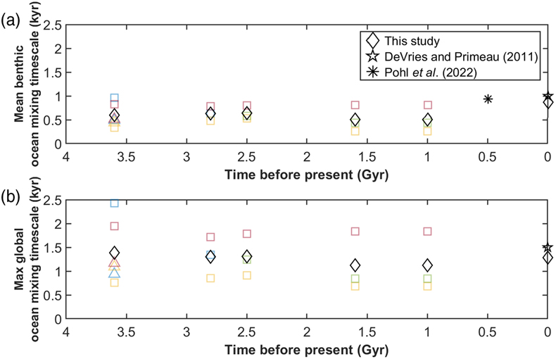
Figure 2 Variation in mean benthic (a) and maximum global (b) ocean mixing timescales through time. Squares and triangles correspond to historical experiments with surface pressure of 1 bar and 2 bar, respectively. Continental configuration is represented by blue (aquaplanet), yellow (low latitude supercontinent), red (high latitude supercontinents), and green (Pangaea) symbols. The black diamond at 0 Gyr is our present day baseline experiment, while black diamonds for the historical periods give the mean values of all experiments in the respective period. The asterisk at 0.5 Gyr is modelled Phanerozoic mean benthic ventilation age from Pohl et al. (2022)
Pohl, A., Ridgwell, A., Stockey, R.G., Thomazo, C., Keane, A., Vennin, E., Scotese, C.R. (2022) Continental configuration controls ocean oxygenation during the Phanerozoic. Nature 608, 523–527. https://doi.org/10.1038/s41586-022-05018-z
, and the pentagrams at 0 Gyr are data constrained model estimates of present day ventilation ages from DeVries and Primeau (2011)DeVries, T., Primeau, F. (2011) Dynamically and observationally constrained estimates of water-mass distributions and ages in the global ocean. Journal of Physical Oceanography 41, 2381–2401. https://doi.org/10.1175/JPO-D-10-05011.1
.
Figure 3 (a) Temporal evolution of ɛNd of Precambrian BIFs (black circles; Hu et al., 2020
Hu, J., Wang, H., Zhang, L. (2020) A rare earth element and Nd isotopic investigation into the provenance and deposition of the Dahongliutan banded iron formation and associated carbonates, NW China: Implications on Neoproterozoic seawater compositions. Precambrian Research 342, 105685. https://doi.org/10.1016/j.precamres.2020.105685
; Haugaard et al., 2016Haugaard, R., Ootes, L., Creaser, R.A., Konhauser, K.O. (2016) The nature of Mesoarchaean seawater and continental weathering in 2.85 Ga banded iron formation, Slave craton, NW Canada. Geochimica et Cosmochimica Acta 194, 34–56. https://doi.org/10.1016/j.gca.2016.08.020
), depleted mantle-derived basalts (orange squares; Vervoort and Blichert-Toft, 1999Vervoort, J.D., Blichert-Toft, J. (1999) Evolution of the depleted mantle: Hf isotope evidence from juvenile rocks through time. Geochimica et Cosmochimica Acta 63, 533–556. https://doi.org/10.1016/S0016-7037(98)00274-9
) and detrital sedimentary rocks (blue triangles; Garçon, 2021Garçon, M. (2021) Episodic growth of felsic continents in the past 3.7 Ga. Science Advances 7, eabj1807. https://doi.org/10.1126/sciadv.abj1807
). Archean Superior-type BIFs are represented by black filled circles in the zoom-in view. (b) Modelled seawater ɛNd averaged over various column depths in the Archean ocean with mean benthic ventilation age of 0.33 kyr. The four scenarios are detailed in the main text and Supplementary Information.