



Mercury isotopes in North Pacific sediments reveal vegetation expansion in warm climates
Affiliations | Corresponding Author | Cite as | Funding information
Published by the European Association of Geochemistry
under Creative Commons License CC BY-NC-ND 4.0
Keywords: mercury isotopes, terrestrial vegetation expansion, global mercury cycle, early Holocene, warm Pliocene


- Share this article


-
Article views:1,372Cumulative count of HTML views and PDF downloads.
- Download Citation
- Rights & Permissions

top
Abstract
Figures
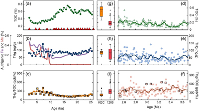 Figure 1 The geochemical data of the Shatsky Rise sediment. (a–c) The geochemical data of core KEC, including the TOC concentration, THg (blue circles) in comparison with authigenic Fe (purple) and Mn (red lines) concentration, and THg/TOC ratio. The red triangles in (a) indicate age control points by 14C dating (see details in Supplementary Information). The bold brown line in (c) is the regression line of the 5-point LOESS smoothing of THg/TOC. (d–f) The geochemical data of Site 1208, including the TOC concentration, THg, and THg/TOC ratio. The bold lines in (d–f) are regression lines with 12-point LOESS smoothing. Squares outlined in black denote samples analysed for Hg isotopes. (g–i) Box-plots comparing the TOC, THg, THg/TOC data between core KEC and Site 1208. | 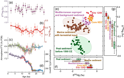 Figure 2 The Hg isotope data of the Shatsky Rise sediment. (a,b) The δ202Hg and Δ199Hg records. Error bars represent the 2 s.d. measurement uncertainty, which are 0.10 ‰ and 0.05 ‰ for δ202Hg and Δ199Hg, respectively. The dark red bold line is the regression line of 5-point LOESS smoothing of Δ199Hg. (c,d) The atmosphere CO2 concentration and δ13Catm recorded in ice cores (Schmitt et al., 2012). The thick lines represent the weighted average across different sites and approaches as indicated by different symbols. (e) The Hg isotope data of this study are compared with a compilation of published pre-anthropogenic Hg data. The Hg isotope data of core KEC and Site 1208 are in orange and red, respectively. Brown symbols are samples from the Arctic Ocean (Gleason et al., 2017) and the South Atlantic Ocean (Figueiredo et al., 2022), which are known to receive direct terrestrial input. Purple symbols are Mediterranean sediments (Gehrke et al., 2009). Peat sediments (Enrico et al., 2017; Li et al., 2023) deposited before 1500 AD are summarised as natural terrestrial Hg isotope endmember. (f,g) Box-plots comparing the dataset shown in (e). | 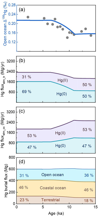 Figure 3 Modelling output illustrating the impact of enhanced atmospheric Hg(0) uptake by the terrestrial system during the early Holocene. (a) The observed (grey points) and model output (blue lines) of the open ocean Δ199Hg. (b) The atmospheric Hg deposition flux to the terrestrial system, with the blue and purple shades indicating Hg(0) and Hg(II) deposition flux, respectively. The percentages indicate the relative contribution of Hg(0) and Hg(II). (c) The atmospheric Hg deposition flux to the open ocean. The shades and percentages are the same as the second row. (d) The Hg burial flux and burial ratio through terrestrial (brown), coastal (yellow), and open ocean (blue) systems. |
| Figure 1 | Figure 2 | Figure 3 |
top
Introduction
Sedimentary mercury (Hg) concentrations and isotope compositions are widely employed as volcanism proxies in palaeoenvironmental studies (Grasby et al., 2019
Grasby, S.E., Them, T.R., Chen, Z., Yin, R., Ardakani, O.H. (2019) Mercury as a proxy for volcanic emissions in the geologic record. Earth-Science Reviews 196, 102880. https://doi.org/10.1016/j.earscirev.2019.102880
). The ratio of total mercury (THg) to total organic carbon (TOC) in sediments is suggested to reflect the changes in seawater Hg concentration and thus the atmospheric Hg load (Grasby et al., 2019Grasby, S.E., Them, T.R., Chen, Z., Yin, R., Ardakani, O.H. (2019) Mercury as a proxy for volcanic emissions in the geologic record. Earth-Science Reviews 196, 102880. https://doi.org/10.1016/j.earscirev.2019.102880
). Mercury isotopes exhibit both significant mass dependent (MDF) and mass independent fractionations (MIF) in natural systems, with the latter primarily generated through specific photochemical reactions (Blum et al., 2014Blum, J.D., Sherman, L.S., Johnson, M.W. (2014) Mercury Isotopes in Earth and Environmental Sciences. Annual Review of Earth and Planetary Sciences 42, 249–269. https://doi.org/10.1146/annurev-earth-050212-124107
). Of particular interest, the odd MIF imparts negative Δ199Hg values to atmosphere gaseous Hg(0) and positive values to oxidised Hg(II). Consequently, the terrestrial and open ocean Hg pools, sourced predominantly from atmospheric Hg(0) and Hg(II), exhibit negative and positive Δ199Hg signatures, respectively (Jiskra et al., 2021Jiskra, M., Heimbürger-Boavida, L.E., Desgranges, M.M., Petrova, M.V., Dufour, A., Ferreira-Araujo, B., Masbou, J., Chmeleff, J., Thyssen, M., Point, D., Sonke, J.E. (2021) Mercury stable isotopes constrain atmospheric sources to the ocean. Nature 597, 678–682. https://doi.org/10.1038/s41586-021-03859-8
; Wang et al., 2022Wang, X., Yuan, W., Lin, C.-J., Feng, X. (2022) Mercury cycling and isotopic fractionation in global forests. Critical Reviews in Environmental Science and Technology 52, 3763–3786. https://doi.org/10.1080/10643389.2021.1961505
).Open ocean Hg burial is primarily driven by sinking particulate organic matter (POM) produced in the surface ocean. As POM sinks and degrades, the Hg bound to POC continuously exchanges with deep water through a process known as “regenerative scavenging” (Lamborg et al., 2016
Lamborg, C.H., Hammerschmidt, C.R., Bowman, K.L. (2016) An examination of the role of particles in oceanic mercury cycling. Philosophical Transactions of the Royal Society A: Mathematical, Physical and Engineering Sciences 374, 20150297. https://doi.org/10.1098/rsta.2015.0297
). Since the inorganic Hg is the dominant Hg form in seawater (Bowman et al., 2020Bowman, K.L., Lamborg, C.H., Agather, A.M. (2020) A global perspective on mercury cycling in the ocean. Science of the Total Environment 710, 136166. https://doi.org/10.1016/j.scitotenv.2019.136166
), the Hg MIF preserved in open ocean sediments (mostly inorganic Hg) is interpreted to represent that of total Hg in the open ocean (Figueiredo et al., 2022Figueiredo, T.S., Bergquist, B.A., Santos, T.P., Albuquerque, A.L.S., Silva-Filho, E.V. (2022) Relationship between glacial CO2 drawdown and mercury cycling in the western South Atlantic: An isotopic insight. Geology 50, 801–805. https://doi.org/10.1130/G49942.1
). Although the Hg-based proxies have been widely used in palaeoclimate research, the potential reorganisation of the global Hg cycle under different climate regimes remains to be constrained.Here we present sedimentary records of open ocean Hg concentration and isotope compositions across contrasting climate states. The sediment records are recovered from Shatsky Rise in the North Pacific open ocean, a remote region far from the continental shelf and receiving minimal direct terrestrial input. A previous study indicates that its sedimentary organic matter is predominantly marine sourced (Maeda et al., 2002
Maeda, L., Kawahata, H., Nohara, M. (2002) Fluctuation of biogenic and abiogenic sedimentation on the Shatsky Rise in the western North Pacific during the late Quaternary. Marine Geology 189, 197–214. https://doi.org/10.1016/S0025-3227(02)00405-X
). Dissolved Hg in the deep Northwest Pacific reflects both the deep water source signatures as well as the accumulation resulting from release during organic carbon remineralisation along the global ocean conveyer belt (Zhang et al., 2014Zhang, Y., Jaeglé, L., Thompson, L. (2014) Natural biogeochemical cycle of mercury in a global three‐dimensional ocean tracer model. Global Biogeochemical Cycles 28, 553–570. https://doi.org/10.1002/2014GB004814
). Therefore, the Shatsky Rise sediment has the potential to provide valuable insights into global scale open ocean Hg cycling, while more records from other open ocean sites might help to assess regional variability in the future. Two climate periods without large scale volcanism are examined to assess the response of global Hg cycle to climate change, including the period since the Last Glacial Maximum (LGM, about 26 ka) and the warm Pliocene (3.8–2.5 Ma). The former reflects gradual warming and Earth system adjustments, while the latter represents the most recent period significantly warmer than the last glacial-interglacial cycle.top
Materials and Methods
Sediment samples were recovered from Shatsky Rise in the North Pacific open ocean (36.13° N, 158.21° E, water depth of 3346 m). Gravity core KEC records the period since the LGM, whereas ODP Site 1208 archives the warm Pliocene period. Concentrations of total mercury and total organic carbon were determined, with relative standard deviations (RSD) less than 5 % and 2 %, respectively. The easily reducible Fe-Mn oxides are leached, which mainly represent authigenic Fe and Mn oxides in the Shatsky Rise sediment (Qu et al., 2024
Qu, Y., Zhong, H., Liu, X., Zhang, W., Chen, T. (2024) Coupling and Decoupling Between Sedimentary Mercury and Organic Carbon Preservation in the Oxygenated Marine Environment. Geochemistry, Geophysics, Geosystems 25, e2023GC011201. https://doi.org/10.1029/2023GC011201
). The Hg isotope compositions were measured in Tianjin University, with 2 s.d. uncertainty for δ202Hg, Δ199Hg and Δ200Hg of 0.10 ‰, 0.05 ‰, and 0.04 ‰, respectively. To evaluate the response of the global Hg cycle to climate changes, we adapted a five-box model comprising atmospheric Hg(0) and Hg(II) reservoirs, a terrestrial reservoir, and a coastal and open ocean reservoir. Detailed information on samples, analytical protocols, and model configuration is provided in the Supplementary Information.top
Results
In the record since the LGM, the TOC concentration is higher during the glacial period (26–11 ka) than the Holocene (11–0 ka) (Fig. 1). An increase in authigenic Fe and Mn oxide concentrations is observed during the Holocene, when THg exhibits large variations and the THg/TOC ratio increases (Fig. 1b,c). Compared to core KEC, the warm Pliocene record displays lower TOC and THg concentrations but a slightly higher and more variable THg/TOC ratio.
Figure 1 The geochemical data of the Shatsky Rise sediment. (a–c) The geochemical data of core KEC, including the TOC concentration, THg (blue circles) in comparison with authigenic Fe (purple) and Mn (red lines) concentration, and THg/TOC ratio. The red triangles in (a) indicate age control points by 14C dating (see details in Supplementary Information). The bold brown line in (c) is the regression line of the 5-point LOESS smoothing of THg/TOC. (d–f) The geochemical data of Site 1208, including the TOC concentration, THg, and THg/TOC ratio. The bold lines in (d–f) are regression lines with 12-point LOESS smoothing. Squares outlined in black denote samples analysed for Hg isotopes. (g–i) Box-plots comparing the TOC, THg, THg/TOC data between core KEC and Site 1208.
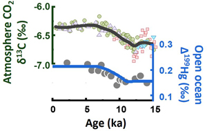
The Hg isotope data for core KEC and Site 1208 are shown in Figure 2. The δ202Hg for core KEC has no long-term trend since the LGM (Fig. 2a). The Δ199Hg rises during the early Holocene (11–8 ka), and is significantly higher in the mid- to late Holocene (8–0 ka; 0.21 ± 0.03 ‰, 2 s.d., n = 5) than in the glacial period (26–11 ka; 0.16 ± 0.06 ‰, 2 s.d., n = 14; unpaired Wilcoxon test, p < 0.05). For Site 1208, the δ202Hg and Δ199Hg exhibit no secular change. The average Δ199Hg of Site 1208 samples for the Pliocene is 0.06 ‰ higher (unpaired Wilcoxon test, p < 0.05) than that of core KEC samples since the LGM (0.23 ‰ vs. 0.17 ‰) (Fig. 2g). The Δ200Hg shows no secular change and has no systematical difference between core KEC and Site 1208 sediments. Details on Hg isotope data are provided in the Supplementary Information.
Figure 2 The Hg isotope data of the Shatsky Rise sediment. (a,b) The δ202Hg and Δ199Hg records. Error bars represent the 2 s.d. measurement uncertainty, which are 0.10 ‰ and 0.05 ‰ for δ202Hg and Δ199Hg, respectively. The dark red bold line is the regression line of 5-point LOESS smoothing of Δ199Hg. (c,d) The atmosphere CO2 concentration and δ13Catm recorded in ice cores (Schmitt et al., 2012
Schmitt, J., Schneider, R., Elsig, J., Leuenberger, D., Lourantou, A., Chappellaz, J., Köhler, P., Joos, F., Stocker, T.F., Leuenberger, M., Fischer, H. (2012) Carbon Isotope Constraints on the Deglacial CO2 Rise from Ice Cores. Science 336, 711–714. https://doi.org/10.1126/science.1217161
). The thick lines represent the weighted average across different sites and approaches as indicated by different symbols. (e) The Hg isotope data of this study are compared with a compilation of published pre-anthropogenic Hg data. The Hg isotope data of core KEC and Site 1208 are in orange and red, respectively. Brown symbols are samples from the Arctic Ocean (Gleason et al., 2017Gleason, J.D., Blum, J.D., Moore, T.C., Polyak, L., Jakobsson, M., Meyers, P.A., Biswas, A. (2017) Sources and cycling of mercury in the paleo Arctic Ocean from Hg stable isotope variations in Eocene and Quaternary sediments. Geochimica et Cosmochimica Acta 197, 245–262. https://doi.org/10.1016/j.gca.2016.10.033
) and the South Atlantic Ocean (Figueiredo et al., 2022Figueiredo, T.S., Bergquist, B.A., Santos, T.P., Albuquerque, A.L.S., Silva-Filho, E.V. (2022) Relationship between glacial CO2 drawdown and mercury cycling in the western South Atlantic: An isotopic insight. Geology 50, 801–805. https://doi.org/10.1130/G49942.1
), which are known to receive direct terrestrial input. Purple symbols are Mediterranean sediments (Gehrke et al., 2009Gehrke, G.E., Blum, J.D., Meyers, P.A. (2009) The geochemical behavior and isotopic composition of Hg in a mid-Pleistocene western Mediterranean sapropel. Geochimica et Cosmochimica Acta 73, 1651–1665. https://doi.org/10.1016/j.gca.2008.12.012
). Peat sediments (Enrico et al., 2017Enrico, M., Le Roux, G., Heimbürger, L.-E., Van Beek, P., Souhaut, M., Chmeleff, J., Sonke, J.E. (2017) Holocene Atmospheric Mercury Levels Reconstructed from Peat Bog Mercury Stable Isotopes. Environmental Science & Technology 51, 5899–5906. https://doi.org/10.1021/acs.est.6b05804
; Li et al., 2023Li, C., Jiskra, M., Nilsson, M.B., Osterwalder, S., Zhu, W., Mauquoy, D., Skyllberg, U., Enrico, M., Peng, H., Song, Y., Björn, E., Bishop, K. (2023) Mercury deposition and redox transformation processes in peatland constrained by mercury stable isotopes. Nature Communications 14, 7389. https://doi.org/10.1038/s41467-023-43164-8
) deposited before 1500 AD are summarised as natural terrestrial Hg isotope endmember. (f,g) Box-plots comparing the dataset shown in (e).top
Discussion
Higher sedimentary Δ 199 Hg during warm climate states . In the record since the LGM, the lower TOC and higher authigenic Fe and Mn oxides (Fig. 1) indicate lower productivity and higher bottom water oxygenation during Holocene than the glacial period (Maeda et al., 2002
Maeda, L., Kawahata, H., Nohara, M. (2002) Fluctuation of biogenic and abiogenic sedimentation on the Shatsky Rise in the western North Pacific during the late Quaternary. Marine Geology 189, 197–214. https://doi.org/10.1016/S0025-3227(02)00405-X
; Galbraith et al., 2007Galbraith, E.D., Jaccard, S.L., Pedersen, T.F., Sigman, D.M., Haug, G.H., Cook, M., Southon, J.R., Francois, R. (2007) Carbon dioxide release from the North Pacific abyss during the last deglaciation. Nature 449, 890–893. https://doi.org/10.1038/nature06227
). In the oxic Holocene sediment, the THg/TOC ratio has a higher value and larger variability than the glacial period due to the early diagenetic effect (Qu et al., 2024Qu, Y., Zhong, H., Liu, X., Zhang, W., Chen, T. (2024) Coupling and Decoupling Between Sedimentary Mercury and Organic Carbon Preservation in the Oxygenated Marine Environment. Geochemistry, Geophysics, Geosystems 25, e2023GC011201. https://doi.org/10.1029/2023GC011201
). Similar phenomenon in THg/TOC ratio is also observed in the warm Pliocene sediment (Fig. 1f) with high bottom water oxygenation (Abell and Winckler, 2023Abell, J.T., Winckler, G. (2023) Long-Term Variability in Pliocene North Pacific Ocean Export Production and Its Implications for Ocean Circulation in a Warmer World. AGU Advances 4, e2022AV000853. https://doi.org/10.1029/2022AV000853
). The diagenetic mobilisation of Hg prohibits using THg/TOC and δ202Hg to reliably record past seawater signatures. However, the sedimentary Δ199Hg has been shown to be resistant to diagenesis, thus mostly retaining the seawater signal (Chen et al., 2022Chen, D., Ren, D., Deng, C., Tian, Z., Yin, R. (2022) Mercury loss and isotope fractionation during high-pressure and high-temperature processing of sediments: Implication for the behaviors of mercury during metamorphism. Geochimica et Cosmochimica Acta 334, 231–240. https://doi.org/10.1016/j.gca.2022.08.010
).The observed Δ199Hg values in Shatsky Rise sediment are significantly higher than those reported for pre-anthropogenic marine sediments deposited along continental margins (Fig. 2e) (Gehrke et al., 2009
Gehrke, G.E., Blum, J.D., Meyers, P.A. (2009) The geochemical behavior and isotopic composition of Hg in a mid-Pleistocene western Mediterranean sapropel. Geochimica et Cosmochimica Acta 73, 1651–1665. https://doi.org/10.1016/j.gca.2008.12.012
; Gleason et al., 2017Gleason, J.D., Blum, J.D., Moore, T.C., Polyak, L., Jakobsson, M., Meyers, P.A., Biswas, A. (2017) Sources and cycling of mercury in the paleo Arctic Ocean from Hg stable isotope variations in Eocene and Quaternary sediments. Geochimica et Cosmochimica Acta 197, 245–262. https://doi.org/10.1016/j.gca.2016.10.033
; Figueiredo et al., 2022Figueiredo, T.S., Bergquist, B.A., Santos, T.P., Albuquerque, A.L.S., Silva-Filho, E.V. (2022) Relationship between glacial CO2 drawdown and mercury cycling in the western South Atlantic: An isotopic insight. Geology 50, 801–805. https://doi.org/10.1130/G49942.1
), suggesting little influence from terrestrial input of negative Δ199Hg. Given its open ocean setting, the Shatsky Rise has the potential to provide an open ocean Δ199Hg reference value, and most likely records the open ocean Δ199Hg evolution through climate changes (see details in the Supplementary Information). The most prominent feature of the Δ199Hg record since the LGM is the clear increasing trend during the early Holocene (∼11 to 8 ka), which is similar to the rise in atmosphere CO2 carbon isotope (δ13Catm) (Fig. 2b,c). The deglacial atmospheric CO2 (pCO2) increase results in a warmer and wetter climate in the early Holocene, which promotes the expansion of terrestrial vegetation (Prentice et al., 2011Prentice, I.C., Harrison, S.P., Bartlein, P.J. (2011) Global vegetation and terrestrial carbon cycle changes after the last ice age. New Phytologist 189, 988–998. https://doi.org/10.1111/j.1469-8137.2010.03620.x
; Ciais et al., 2012Ciais, P., Tagliabue, A., Cuntz, M., Bopp, L., Scholze, M., Hoffmann, G., Lourantou, A., Harrison, S.P., Prentice, I.C., Kelley, D.I., Koven, C., Piao, S.L. (2012) Large inert carbon pool in the terrestrial biosphere during the Last Glacial Maximum. Nature Geoscience 5, 74–79. https://doi.org/10.1038/ngeo1324
). The enhanced terrestrial productivity preferentially assimilates the lighter carbon isotope (12C relative to 13C) from the atmosphere and leads to the δ13Catm increase. The same process has been shown to increase terrestrial uptake of Hg(0) (Jiskra et al., 2018Jiskra, M., Sonke, J.E., Obrist, D., Bieser, J., Ebinghaus, R., Myhre, C.L., Pfaffhuber, K.A., Wängberg, I., Kyllönen, K., Worthy, D., Martin, L.G., Labuschagne, C., Mkololo, T., Ramonet, M., Magand, O., Dommergue, A. (2018) A vegetation control on seasonal variations in global atmospheric mercury concentrations. Nature Geoscience 11, 244–250. https://doi.org/10.1038/s41561-018-0078-8
), characterised by a negative Δ199Hg value. Therefore, the increased terrestrial Hg fixation and burial would elevate the Δ199Hg of the atmosphere and open ocean system considering the mass balance of Hg isotopes in the whole Earth surface system.Water column processes, including methylmercury degradation and Hg(II) reduction, may also have an influence on the Δ199Hg signature of the open ocean Hg and thus the sediment record. However, if these processes were the primary driver of sedimentary Δ199Hg evolution, the record would be expected to follow the glacial-interglacial changes in environmental factors in the northwest Pacific (Rae et al., 2020
Rae, J.W.B., Gray, W.R., Wills, R.C.J., Eisenman, I., Fitzhugh, B., Fotheringham, M., Littley, E.F.M., Rafter, P.A., Rees-Owen, R., Ridgwell, A., Taylor, B., Burke, A. (2020) Overturning circulation, nutrient limitation, and warming in the Glacial North Pacific. Science Advances 6, eabd1654. https://doi.org/10.1126/sciadv.abd1654
), such as solar radiation, dissolved oxygen, and productivity. The absence of a distinct Δ199Hg shift during deglaciation, coupled with its co-variation with δ13Catm during the Holocene (11–0 ka) (ρ = 0.85, p < 0.05; Spearman’s rank correlation analysis), suggests that water column processes are likely not the primary drivers. The Δ200Hg versus Δ199Hg relationship further supports limited net MIF in the water column, where the sedimentary data are mostly on the mixing line of atmospheric Hg(0) and Hg(II) sources (see details in the Supplementary Information). The open ocean Δ199Hg signature is thus dictated by its major source, the atmospheric Hg(0) and Hg(II) deposition (Jiskra et al., 2021Jiskra, M., Heimbürger-Boavida, L.E., Desgranges, M.M., Petrova, M.V., Dufour, A., Ferreira-Araujo, B., Masbou, J., Chmeleff, J., Thyssen, M., Point, D., Sonke, J.E. (2021) Mercury stable isotopes constrain atmospheric sources to the ocean. Nature 597, 678–682. https://doi.org/10.1038/s41586-021-03859-8
), followed by transport to the deep ocean through deep water formation and POM remineralisation, and deposition in the sedimentary matter. Therefore, the increasing Δ199Hg observed in Shatsky Rise sediments during the early Holocene can be well explained by elevated atmospheric Δ199Hg due to enhanced terrestrial vegetation growth and associated Hg sequestration.Another typical warm climate state is the Pliocene when there was limited Northern Hemisphere Glaciation (Fedorov et al., 2013
Fedorov, A.V., Brierley, C.M., Lawrence, K.T., Liu, Z., Dekens, P.S., Ravelo, A.C. (2013) Patterns and mechanisms of early Pliocene warmth. Nature 496, 43–49. https://doi.org/10.1038/nature12003
). The terrestrial vegetation was more productive and the arid areas such as deserts were smaller during the warm Pliocene when the Northern Hemisphere was covered by high-latitude forests rather than the modern tundra-type vegetation (Haywood and Valdes, 2006Haywood, A.M., Valdes, P.J. (2006) Vegetation cover in a warmer world simulated using a dynamic global vegetation model for the Mid-Pliocene. Palaeogeography, Palaeoclimatology, Palaeoecology 237, 412–427. https://doi.org/10.1016/j.palaeo.2005.12.012
). The open ocean Δ199Hg recorded by Shatsky Rise sediment is also higher (unpaired Wilcoxon test, p < 0.05) during the warm Pliocene (Δ199Hg = 0.23 ± 0.09 ‰, 2 s.d., n = 11) than the period since the LGM (Δ199Hg = 0.17 ± 0.06 ‰, 2 s.d., n = 25). The comparison of the two climate states reveals a consistently higher open ocean Δ199Hg during warmer climates when terrestrial vegetation productivity is enhanced. In the following, we will use a time-dependent atmosphere-terrestrial-ocean box model to quantitatively explore the mechanism for the observed Δ199Hg changes.Modelling representation of natural Hg cycles. Using the simplified Hg isotope box model, we first test whether the observed Δ199Hg shift could be explained by enhanced Hg(0) uptake by the terrestrial vegetation system. Given that atmospheric and oceanic circulation may experience adjustment during the early Holocene, other scenarios that could affect open ocean Δ199Hg are also explored, including increased atmospheric Hg(II) deposition to the open ocean, decreased sedimental Hg burial efficiency in open ocean, and decreased coastal to open ocean connectivity due to sea level rising.
By using well constrained parameters (sizes of reservoirs, fluxes between reservoirs, and isotope fractionation factors of Δ199Hg), the model is set as steady states during the late Holocene and the deglacial, and all perturbations in different simulation scenarios are introduced during the early Holocene. Modelling details are provided in the Supplementary Information. In the first scenario, the model prescribes that vegetation Hg(0) uptake contributes about 70 % of the terrestrial Hg fixation relative to about 30 % from atmospheric Hg(II) in the late Holocene, based on modern observations (Wang et al., 2022
Wang, X., Yuan, W., Lin, C.-J., Feng, X. (2022) Mercury cycling and isotopic fractionation in global forests. Critical Reviews in Environmental Science and Technology 52, 3763–3786. https://doi.org/10.1080/10643389.2021.1961505
). The atmospheric Hg(0) deposition flux into the vegetation before the early Holocene is set at a low value to account for the change in terrestrial biosphere since the early Holocene. The result suggests that enhanced terrestrial Hg(0) uptake flux by a factor of 1.7 relative to the deglacial steady state could broadly reproduce the observed Δ199Hg shift during the early Holocene (Fig. 3a). This is consistent with previous studies of the δ13Catm record and modelling results, which suggest that the expansion of the terrestrial biosphere during the early Holocene (Schmitt et al., 2012Schmitt, J., Schneider, R., Elsig, J., Leuenberger, D., Lourantou, A., Chappellaz, J., Köhler, P., Joos, F., Stocker, T.F., Leuenberger, M., Fischer, H. (2012) Carbon Isotope Constraints on the Deglacial CO2 Rise from Ice Cores. Science 336, 711–714. https://doi.org/10.1126/science.1217161
) increased the terrestrial primary productivity by a factor of 1.43 to 2.00 (Prentice et al., 2011Prentice, I.C., Harrison, S.P., Bartlein, P.J. (2011) Global vegetation and terrestrial carbon cycle changes after the last ice age. New Phytologist 189, 988–998. https://doi.org/10.1111/j.1469-8137.2010.03620.x
; Ciais et al., 2012Ciais, P., Tagliabue, A., Cuntz, M., Bopp, L., Scholze, M., Hoffmann, G., Lourantou, A., Harrison, S.P., Prentice, I.C., Kelley, D.I., Koven, C., Piao, S.L. (2012) Large inert carbon pool in the terrestrial biosphere during the Last Glacial Maximum. Nature Geoscience 5, 74–79. https://doi.org/10.1038/ngeo1324
).Figure 3 Modelling output illustrating the impact of enhanced atmospheric Hg(0) uptake by the terrestrial system during the early Holocene. (a) The observed (grey points) and model output (blue lines) of the open ocean Δ199Hg. (b) The atmospheric Hg deposition flux to the terrestrial system, with the blue and purple shades indicating Hg(0) and Hg(II) deposition flux, respectively. The percentages indicate the relative contribution of Hg(0) and Hg(II). (c) The atmospheric Hg deposition flux to the open ocean. The shades and percentages are the same as the second row. (d) The Hg burial flux and burial ratio through terrestrial (brown), coastal (yellow), and open ocean (blue) systems.
In the second and third scenarios, the increase in atmospheric Hg(II) deposition flux and the decreased Hg burial in the open ocean are considered during the early Holocene. To reproduce the observed Δ199Hg shift, large variations in precipitation (2.4×) or POM-related open ocean Hg burial flux (0.6×) are needed during the early Holocene, which are not supported by previous studies (Cartapanis et al., 2016
Cartapanis, O., Bianchi, D., Jaccard, S.L., Galbraith, E.D. (2016) Global pulses of organic carbon burial in deep-sea sediments during glacial maxima. Nature Communications 7, 10796. https://doi.org/10.1038/ncomms10796
; Hancock et al., 2023Hancock, C.L., McKay, N.P., Erb, M.P., Kaufman, D.S., Routson, C.R., Ivanovic, R.F., Gregoire, L.J., Valdes, P. (2023) Global Synthesis of Regional Holocene Hydroclimate Variability Using Proxy and Model Data. Paleoceanography and Paleoclimatology 38, e2022PA004597. https://doi.org/10.1029/2022PA004597
). In the fourth scenario, Hg transport flux from the coastal to open ocean decreased by a factor of 0.33. However, the deglacial sea level rise and the associated decrease in coastal-open ocean connectivity starts at about 17.5 ka (Yokoyama et al., 2018Yokoyama, Y., Esat, T.M., Thompson, W.G., Thomas, A.L., Webster, J.M., Miyairi, Y., Sawada, C., Aze, T., Matsuzaki, H., Okuno, J., Fallon, S., Braga, J., Humblet, M., Iryu, Y., Potts, D.C., Fujita, K., Suzuki, A., Kan, H. (2018) Rapid glaciation and a two-step sea level plunge into the Last Glacial Maximum. Nature 559, 603–607. https://doi.org/10.1038/s41586-018-0335-4
), predating the observed Δ199Hg increase. The timing thus precludes the change in coastal to open ocean Hg transport as the prominent driver of open ocean Δ199Hg shift. Based on the open ocean Δ199Hg record and the four modelling scenarios, we suggest that the early Holocene Δ199Hg increase is most probably caused by increased Hg(0) uptake by the terrestrial ecosystem.top
Conclusions and Implications
The Hg isotope record from North Pacific open ocean sediments at the Shatsky Rise reveals elevated Δ199Hg values during warm periods, including the mid- to late Holocene and the warm Pliocene. Using a simplified Hg isotope box model, we propose that the expansion of the terrestrial biosphere is likely the primary driver of this pattern, highlighting the significant role of terrestrial vegetation in the global Hg cycle. Previous research on modern atmospheric Hg(0) indicates that vegetation uptake of Hg(0) is a crucial factor in regulating Hg distribution between the atmosphere and terrestrial system on a seasonal timescale (Jiskra et al., 2018
Jiskra, M., Sonke, J.E., Obrist, D., Bieser, J., Ebinghaus, R., Myhre, C.L., Pfaffhuber, K.A., Wängberg, I., Kyllönen, K., Worthy, D., Martin, L.G., Labuschagne, C., Mkololo, T., Ramonet, M., Magand, O., Dommergue, A. (2018) A vegetation control on seasonal variations in global atmospheric mercury concentrations. Nature Geoscience 11, 244–250. https://doi.org/10.1038/s41561-018-0078-8
). This work suggests that the vegetation uptake of Hg(0) might also be the dominant factor driving the global Hg cycle across various climate states on a longer timescale. In the context of global change, the responses of terrestrial Hg and carbon cycles remain unclear due to the intricate mechanisms governing terrestrial ecosystem responses (Luo, 2007Luo, Y. (2007) Terrestrial carbon-cycle feedback to climate warming. Annual Review of Ecology, Evolution, and Systematics 38, 683–712. https://doi.org/10.1146/annurev.ecolsys.38.091206.095808
). By showing enhanced terrestrial productivity and Hg and carbon stocks during past warm climate states, our study offers insights into potential future responses. With the forest ecosystem restoration (Watson et al., 2018Watson, J.E.M., Evans, T., Venter, O., Williams, B., Tulloch, A., Stewart, C., Thompson, I., Ray, J.C., Murray, K., Salazar, A., McAlpine, C., Potapov, P., Walston, J., Robinson, J.G., Painter, M., Wilkie, D., Filardi, C., Laurance, W.F., Houghton, R.A., Maxwell, S., Grantham, H., Samper, C., Wang, S., Laestadius, L., Runting, R.K., Silva-Chávez, G.A., Ervin, J., Lindenmayer, D. (2018) The exceptional value of intact forest ecosystems. Nature Ecology & Evolution 2, 599–610. https://doi.org/10.1038/s41559-018-0490-x
), the terrestrial biosphere has the potential to store more Hg from the atmosphere and thus alleviate Hg pollution in the open ocean. Additionally, our results highlight the need to consider significant climate and environmental adjustments when using Hg concentrations and isotopes to trace large scale volcanism in the geological history.top
Acknowledgements
We are grateful to the editor and two reviewers for their constructive comments and suggestions. This research is funded by the National Key Research and Development Program of China (2023YFF0805004), and the National Natural Science Foundation of China (41991325, 42373011, 42173081, 42373011). This research used samples and data provided by Ocean Drilling Program (ODP). The KEC samples were collected onboard of R/V Tan Kah Kee implementing the open research cruise NORC2022-306 supported by NSFC Shiptime Sharing Project (project number: 42149303).
Editor: Gavin Foster
top
References
Abell, J.T., Winckler, G. (2023) Long-Term Variability in Pliocene North Pacific Ocean Export Production and Its Implications for Ocean Circulation in a Warmer World. AGU Advances 4, e2022AV000853. https://doi.org/10.1029/2022AV000853
 Show in context
 Similar phenomenon in THg/TOC ratio is also observed in the warm Pliocene sediment (Fig. 1f) with high bottom water oxygenation (Abell and Winckler, 2023).
View in article
Blum, J.D., Sherman, L.S., Johnson, M.W. (2014) Mercury Isotopes in Earth and Environmental Sciences. Annual Review of Earth and Planetary Sciences 42, 249–269. https://doi.org/10.1146/annurev-earth-050212-124107
Show in context Mercury isotopes exhibit both significant mass dependent (MDF) and mass independent fractionations (MIF) in natural systems, with the latter primarily generated through specific photochemical reactions (Blum et al., 2014).
View in article
Bowman, K.L., Lamborg, C.H., Agather, A.M. (2020) A global perspective on mercury cycling in the ocean. Science of the Total Environment 710, 136166. https://doi.org/10.1016/j.scitotenv.2019.136166
Show in context Since the inorganic Hg is the dominant Hg form in seawater (Bowman et al., 2020), the Hg MIF preserved in open ocean sediments (mostly inorganic Hg) is interpreted to represent that of total Hg in the open ocean (Figueiredo et al., 2022).
View in article
Cartapanis, O., Bianchi, D., Jaccard, S.L., Galbraith, E.D. (2016) Global pulses of organic carbon burial in deep-sea sediments during glacial maxima. Nature Communications 7, 10796. https://doi.org/10.1038/ncomms10796
Show in context To reproduce the observed Δ199Hg shift, large variations in precipitation (2.4×) or POM-related open ocean Hg burial flux (0.6×) are needed during the early Holocene, which are not supported by previous studies (Cartapanis et al., 2016; Hancock et al., 2023).
View in article
Chen, D., Ren, D., Deng, C., Tian, Z., Yin, R. (2022) Mercury loss and isotope fractionation during high-pressure and high-temperature processing of sediments: Implication for the behaviors of mercury during metamorphism. Geochimica et Cosmochimica Acta 334, 231–240. https://doi.org/10.1016/j.gca.2022.08.010
Show in context However, the sedimentary Δ199Hg has been shown to be resistant to diagenesis, thus mostly retaining the seawater signal (Chen et al., 2022).
View in article
Ciais, P., Tagliabue, A., Cuntz, M., Bopp, L., Scholze, M., Hoffmann, G., Lourantou, A., Harrison, S.P., Prentice, I.C., Kelley, D.I., Koven, C., Piao, S.L. (2012) Large inert carbon pool in the terrestrial biosphere during the Last Glacial Maximum. Nature Geoscience 5, 74–79. https://doi.org/10.1038/ngeo1324
Show in context The deglacial atmospheric CO2 (pCO2) increase results in a warmer and wetter climate in the early Holocene, which promotes the expansion of terrestrial vegetation (Prentice et al., 2011; Ciais et al., 2012).
View in article
This is consistent with previous studies of the δ13Catm record and modelling results, which suggest that the expansion of the terrestrial biosphere during the early Holocene (Schmitt et al., 2012) increased the terrestrial primary productivity by a factor of 1.43 to 2.00 (Prentice et al., 2011; Ciais et al., 2012).
View in article
Enrico, M., Le Roux, G., Heimbürger, L.-E., Van Beek, P., Souhaut, M., Chmeleff, J., Sonke, J.E. (2017) Holocene Atmospheric Mercury Levels Reconstructed from Peat Bog Mercury Stable Isotopes. Environmental Science & Technology 51, 5899–5906. https://doi.org/10.1021/acs.est.6b05804
Show in context Purple symbols are Mediterranean sediments (Gehrke et al., 2009). Peat sediments (Enrico et al., 2017; Li et al., 2023) deposited before 1500 AD are summarised as natural terrestrial Hg isotope endmember.
View in article
Fedorov, A.V., Brierley, C.M., Lawrence, K.T., Liu, Z., Dekens, P.S., Ravelo, A.C. (2013) Patterns and mechanisms of early Pliocene warmth. Nature 496, 43–49. https://doi.org/10.1038/nature12003
Show in context Another typical warm climate state is the Pliocene when there was limited Northern Hemisphere Glaciation (Fedorov et al., 2013).
View in article
Figueiredo, T.S., Bergquist, B.A., Santos, T.P., Albuquerque, A.L.S., Silva-Filho, E.V. (2022) Relationship between glacial CO2 drawdown and mercury cycling in the western South Atlantic: An isotopic insight. Geology 50, 801–805. https://doi.org/10.1130/G49942.1
Show in context Since the inorganic Hg is the dominant Hg form in seawater (Bowman et al., 2020), the Hg MIF preserved in open ocean sediments (mostly inorganic Hg) is interpreted to represent that of total Hg in the open ocean (Figueiredo et al., 2022).
View in article
Brown symbols are samples from the Arctic Ocean (Gleason et al., 2017) and the South Atlantic Ocean (Figueiredo et al., 2022), which are known to receive direct terrestrial input.
View in article
The observed Δ199Hg values in Shatsky Rise sediment are significantly higher than those reported for pre-anthropogenic marine sediments deposited along continental margins (Fig. 2e) (Gehrke et al., 2009; Gleason et al., 2017; Figueiredo et al., 2022), suggesting little influence from terrestrial input of negative Δ199Hg.
View in article
Galbraith, E.D., Jaccard, S.L., Pedersen, T.F., Sigman, D.M., Haug, G.H., Cook, M., Southon, J.R., Francois, R. (2007) Carbon dioxide release from the North Pacific abyss during the last deglaciation. Nature 449, 890–893. https://doi.org/10.1038/nature06227
Show in context In the record since the LGM, the lower TOC and higher authigenic Fe and Mn oxides (Fig. 1) indicate lower productivity and higher bottom water oxygenation during Holocene than the glacial period (Maeda et al., 2002; Galbraith et al., 2007).
View in article
Gehrke, G.E., Blum, J.D., Meyers, P.A. (2009) The geochemical behavior and isotopic composition of Hg in a mid-Pleistocene western Mediterranean sapropel. Geochimica et Cosmochimica Acta 73, 1651–1665. https://doi.org/10.1016/j.gca.2008.12.012
Show in context Purple symbols are Mediterranean sediments (Gehrke et al., 2009). Peat sediments (Enrico et al., 2017; Li et al., 2023) deposited before 1500 AD are summarised as natural terrestrial Hg isotope endmember.
View in article
The observed Δ199Hg values in Shatsky Rise sediment are significantly higher than those reported for pre-anthropogenic marine sediments deposited along continental margins (Fig. 2e) (Gehrke et al., 2009; Gleason et al., 2017; Figueiredo et al., 2022), suggesting little influence from terrestrial input of negative Δ199Hg.
View in article
Gleason, J.D., Blum, J.D., Moore, T.C., Polyak, L., Jakobsson, M., Meyers, P.A., Biswas, A. (2017) Sources and cycling of mercury in the paleo Arctic Ocean from Hg stable isotope variations in Eocene and Quaternary sediments. Geochimica et Cosmochimica Acta 197, 245–262. https://doi.org/10.1016/j.gca.2016.10.033
Show in context Brown symbols are samples from the Arctic Ocean (Gleason et al., 2017) and the South Atlantic Ocean (Figueiredo et al., 2022), which are known to receive direct terrestrial input.
View in article
The observed Δ199Hg values in Shatsky Rise sediment are significantly higher than those reported for pre-anthropogenic marine sediments deposited along continental margins (Fig. 2e) (Gehrke et al., 2009; Gleason et al., 2017; Figueiredo et al., 2022), suggesting little influence from terrestrial input of negative Δ199Hg.
View in article
Grasby, S.E., Them, T.R., Chen, Z., Yin, R., Ardakani, O.H. (2019) Mercury as a proxy for volcanic emissions in the geologic record. Earth-Science Reviews 196, 102880. https://doi.org/10.1016/j.earscirev.2019.102880
Show in context Sedimentary mercury (Hg) concentrations and isotope compositions are widely employed as volcanism proxies in palaeoenvironmental studies (Grasby et al., 2019).
View in article
The ratio of total mercury (THg) to total organic carbon (TOC) in sediments is suggested to reflect the changes in seawater Hg concentration and thus the atmospheric Hg load (Grasby et al., 2019).
View in article
Hancock, C.L., McKay, N.P., Erb, M.P., Kaufman, D.S., Routson, C.R., Ivanovic, R.F., Gregoire, L.J., Valdes, P. (2023) Global Synthesis of Regional Holocene Hydroclimate Variability Using Proxy and Model Data. Paleoceanography and Paleoclimatology 38, e2022PA004597. https://doi.org/10.1029/2022PA004597
Show in context To reproduce the observed Δ199Hg shift, large variations in precipitation (2.4×) or POM-related open ocean Hg burial flux (0.6×) are needed during the early Holocene, which are not supported by previous studies (Cartapanis et al., 2016; Hancock et al., 2023).
View in article
Haywood, A.M., Valdes, P.J. (2006) Vegetation cover in a warmer world simulated using a dynamic global vegetation model for the Mid-Pliocene. Palaeogeography, Palaeoclimatology, Palaeoecology 237, 412–427. https://doi.org/10.1016/j.palaeo.2005.12.012
Show in context The terrestrial vegetation was more productive and the arid areas such as deserts were smaller during the warm Pliocene when the Northern Hemisphere was covered by high-latitude forests rather than the modern tundra-type vegetation (Haywood and Valdes, 2006).
View in article
Jiskra, M., Sonke, J.E., Obrist, D., Bieser, J., Ebinghaus, R., Myhre, C.L., Pfaffhuber, K.A., Wängberg, I., Kyllönen, K., Worthy, D., Martin, L.G., Labuschagne, C., Mkololo, T., Ramonet, M., Magand, O., Dommergue, A. (2018) A vegetation control on seasonal variations in global atmospheric mercury concentrations. Nature Geoscience 11, 244–250. https://doi.org/10.1038/s41561-018-0078-8
Show in context The same process has been shown to increase terrestrial uptake of Hg(0) (Jiskra et al., 2018), characterised by a negative Δ199Hg value.
View in article
Previous research on modern atmospheric Hg(0) indicates that vegetation uptake of Hg(0) is a crucial factor in regulating Hg distribution between the atmosphere and terrestrial system on a seasonal timescale (Jiskra et al., 2018).
View in article
Jiskra, M., Heimbürger-Boavida, L.E., Desgranges, M.M., Petrova, M.V., Dufour, A., Ferreira-Araujo, B., Masbou, J., Chmeleff, J., Thyssen, M., Point, D., Sonke, J.E. (2021) Mercury stable isotopes constrain atmospheric sources to the ocean. Nature 597, 678–682. https://doi.org/10.1038/s41586-021-03859-8
Show in context Consequently, the terrestrial and open ocean Hg pools, sourced predominantly from atmospheric Hg(0) and Hg(II), exhibit negative and positive Δ199Hg signatures, respectively (Jiskra et al., 2021; Wang et al., 2022).
View in article
The open ocean Δ199Hg signature is thus dictated by its major source, the atmospheric Hg(0) and Hg(II) deposition (Jiskra et al., 2021), followed by transport to the deep ocean through deep water formation and POM remineralisation, and deposition in the sedimentary matter.
View in article
Lamborg, C.H., Hammerschmidt, C.R., Bowman, K.L. (2016) An examination of the role of particles in oceanic mercury cycling. Philosophical Transactions of the Royal Society A: Mathematical, Physical and Engineering Sciences 374, 20150297. https://doi.org/10.1098/rsta.2015.0297
Show in context As POM sinks and degrades, the Hg bound to POC continuously exchanges with deep water through a process known as “regenerative scavenging” (Lamborg et al., 2016).
View in article
Li, C., Jiskra, M., Nilsson, M.B., Osterwalder, S., Zhu, W., Mauquoy, D., Skyllberg, U., Enrico, M., Peng, H., Song, Y., Björn, E., Bishop, K. (2023) Mercury deposition and redox transformation processes in peatland constrained by mercury stable isotopes. Nature Communications 14, 7389. https://doi.org/10.1038/s41467-023-43164-8
Show in context Purple symbols are Mediterranean sediments (Gehrke et al., 2009). Peat sediments (Enrico et al., 2017; Li et al., 2023) deposited before 1500 AD are summarised as natural terrestrial Hg isotope endmember.
View in article
Luo, Y. (2007) Terrestrial carbon-cycle feedback to climate warming. Annual Review of Ecology, Evolution, and Systematics 38, 683–712. https://doi.org/10.1146/annurev.ecolsys.38.091206.095808
Show in context In the context of global change, the responses of terrestrial Hg and carbon cycles remain unclear due to the intricate mechanisms governing terrestrial ecosystem responses (Luo, 2007).
View in article
Maeda, L., Kawahata, H., Nohara, M. (2002) Fluctuation of biogenic and abiogenic sedimentation on the Shatsky Rise in the western North Pacific during the late Quaternary. Marine Geology 189, 197–214. https://doi.org/10.1016/S0025-3227(02)00405-X
Show in context The sediment records are recovered from Shatsky Rise in the North Pacific open ocean, a remote region far from the continental shelf and receiving minimal direct terrestrial input. A previous study indicates that its sedimentary organic matter is predominantly marine sourced (Maeda et al., 2002).
View in article
In the record since the LGM, the lower TOC and higher authigenic Fe and Mn oxides (Fig. 1) indicate lower productivity and higher bottom water oxygenation during Holocene than the glacial period (Maeda et al., 2002; Galbraith et al., 2007).
View in article
Prentice, I.C., Harrison, S.P., Bartlein, P.J. (2011) Global vegetation and terrestrial carbon cycle changes after the last ice age. New Phytologist 189, 988–998. https://doi.org/10.1111/j.1469-8137.2010.03620.x
Show in context The deglacial atmospheric CO2 (pCO2) increase results in a warmer and wetter climate in the early Holocene, which promotes the expansion of terrestrial vegetation (Prentice et al., 2011; Ciais et al., 2012).
View in article
This is consistent with previous studies of the δ13Catm record and modelling results, which suggest that the expansion of the terrestrial biosphere during the early Holocene (Schmitt et al., 2012) increased the terrestrial primary productivity by a factor of 1.43 to 2.00 (Prentice et al., 2011; Ciais et al., 2012).
View in article
Qu, Y., Zhong, H., Liu, X., Zhang, W., Chen, T. (2024) Coupling and Decoupling Between Sedimentary Mercury and Organic Carbon Preservation in the Oxygenated Marine Environment. Geochemistry, Geophysics, Geosystems 25, e2023GC011201. https://doi.org/10.1029/2023GC011201
Show in context The easily reducible Fe-Mn oxides are leached, which mainly represent authigenic Fe and Mn oxides in the Shatsky Rise sediment (Qu et al., 2024).
View in article
In the oxic Holocene sediment, the THg/TOC ratio has a higher value and larger variability than the glacial period due to the early diagenetic effect (Qu et al., 2024).
View in article
Rae, J.W.B., Gray, W.R., Wills, R.C.J., Eisenman, I., Fitzhugh, B., Fotheringham, M., Littley, E.F.M., Rafter, P.A., Rees-Owen, R., Ridgwell, A., Taylor, B., Burke, A. (2020) Overturning circulation, nutrient limitation, and warming in the Glacial North Pacific. Science Advances 6, eabd1654. https://doi.org/10.1126/sciadv.abd1654
Show in context However, if these processes were the primary driver of sedimentary Δ199Hg evolution, the record would be expected to follow the glacial-interglacial changes in environmental factors in the northwest Pacific (Rae et al., 2020), such as solar radiation, dissolved oxygen, and productivity.
View in article
Schmitt, J., Schneider, R., Elsig, J., Leuenberger, D., Lourantou, A., Chappellaz, J., Köhler, P., Joos, F., Stocker, T.F., Leuenberger, M., Fischer, H. (2012) Carbon Isotope Constraints on the Deglacial CO2 Rise from Ice Cores. Science 336, 711–714. https://doi.org/10.1126/science.1217161
Show in context (c,d) The atmosphere CO2 concentration and δ13Catm recorded in ice cores (Schmitt et al., 2012).
View in article
This is consistent with previous studies of the δ13Catm record and modelling results, which suggest that the expansion of the terrestrial biosphere during the early Holocene (Schmitt et al., 2012) increased the terrestrial primary productivity by a factor of 1.43 to 2.00 (Prentice et al., 2011; Ciais et al., 2012).
View in article
Wang, X., Yuan, W., Lin, C.-J., Feng, X. (2022) Mercury cycling and isotopic fractionation in global forests. Critical Reviews in Environmental Science and Technology 52, 3763–3786. https://doi.org/10.1080/10643389.2021.1961505
Show in context Consequently, the terrestrial and open ocean Hg pools, sourced predominantly from atmospheric Hg(0) and Hg(II), exhibit negative and positive Δ199Hg signatures, respectively (Jiskra et al., 2021; Wang et al., 2022).
View in article
In the first scenario, the model prescribes that vegetation Hg(0) uptake contributes about 70 % of the terrestrial Hg fixation relative to about 30 % from atmospheric Hg(II) in the late Holocene, based on modern observations (Wang et al., 2022).
View in article
Watson, J.E.M., Evans, T., Venter, O., Williams, B., Tulloch, A., Stewart, C., Thompson, I., Ray, J.C., Murray, K., Salazar, A., McAlpine, C., Potapov, P., Walston, J., Robinson, J.G., Painter, M., Wilkie, D., Filardi, C., Laurance, W.F., Houghton, R.A., Maxwell, S., Grantham, H., Samper, C., Wang, S., Laestadius, L., Runting, R.K., Silva-Chávez, G.A., Ervin, J., Lindenmayer, D. (2018) The exceptional value of intact forest ecosystems. Nature Ecology & Evolution 2, 599–610. https://doi.org/10.1038/s41559-018-0490-x
Show in context With the forest ecosystem restoration (Watson et al., 2018), the terrestrial biosphere has the potential to store more Hg from the atmosphere and thus alleviate Hg pollution in the open ocean.
View in article
Yokoyama, Y., Esat, T.M., Thompson, W.G., Thomas, A.L., Webster, J.M., Miyairi, Y., Sawada, C., Aze, T., Matsuzaki, H., Okuno, J., Fallon, S., Braga, J., Humblet, M., Iryu, Y., Potts, D.C., Fujita, K., Suzuki, A., Kan, H. (2018) Rapid glaciation and a two-step sea level plunge into the Last Glacial Maximum. Nature 559, 603–607. https://doi.org/10.1038/s41586-018-0335-4
Show in context However, the deglacial sea level rise and the associated decrease in coastal-open ocean connectivity starts at about 17.5 ka (Yokoyama et al., 2018), predating the observed Δ199Hg increase.
View in article
Zhang, Y., Jaeglé, L., Thompson, L. (2014) Natural biogeochemical cycle of mercury in a global three‐dimensional ocean tracer model. Global Biogeochemical Cycles 28, 553–570. https://doi.org/10.1002/2014GB004814
Show in context Dissolved Hg in the deep Northwest Pacific reflects both the deep water source signatures as well as the accumulation resulting from release during organic carbon remineralisation along the global ocean conveyer belt (Zhang et al., 2014).
View in article
top
Supplementary Information
The Supplementary Information includes:
- Sample Information, Methods, and Details on Data
- Tables S-1 to S-3
- Figures S-1 to S-4
- Supplementary Information References
Download the Supplementary Information (PDF)
Figures
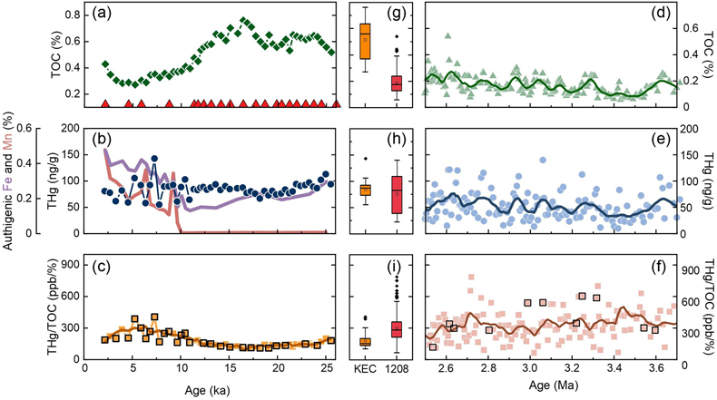
Figure 1 The geochemical data of the Shatsky Rise sediment. (a–c) The geochemical data of core KEC, including the TOC concentration, THg (blue circles) in comparison with authigenic Fe (purple) and Mn (red lines) concentration, and THg/TOC ratio. The red triangles in (a) indicate age control points by 14C dating (see details in Supplementary Information). The bold brown line in (c) is the regression line of the 5-point LOESS smoothing of THg/TOC. (d–f) The geochemical data of Site 1208, including the TOC concentration, THg, and THg/TOC ratio. The bold lines in (d–f) are regression lines with 12-point LOESS smoothing. Squares outlined in black denote samples analysed for Hg isotopes. (g–i) Box-plots comparing the TOC, THg, THg/TOC data between core KEC and Site 1208.
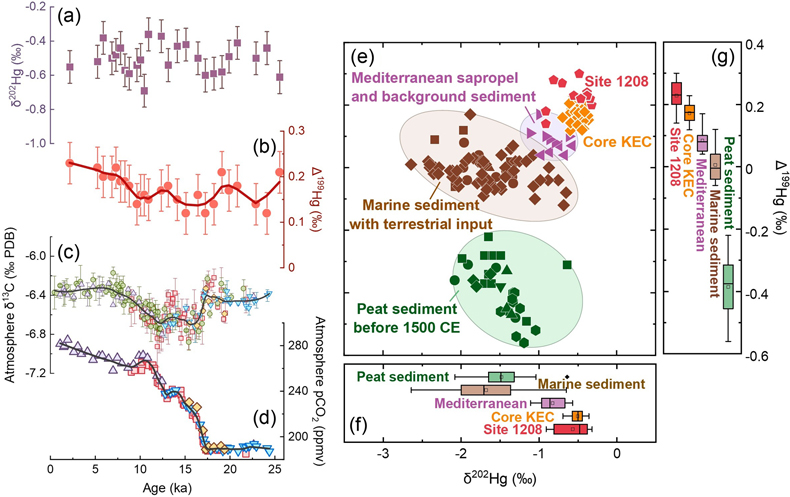
Figure 2 The Hg isotope data of the Shatsky Rise sediment. (a,b) The δ202Hg and Δ199Hg records. Error bars represent the 2 s.d. measurement uncertainty, which are 0.10 ‰ and 0.05 ‰ for δ202Hg and Δ199Hg, respectively. The dark red bold line is the regression line of 5-point LOESS smoothing of Δ199Hg. (c,d) The atmosphere CO2 concentration and δ13Catm recorded in ice cores (Schmitt et al., 2012
Schmitt, J., Schneider, R., Elsig, J., Leuenberger, D., Lourantou, A., Chappellaz, J., Köhler, P., Joos, F., Stocker, T.F., Leuenberger, M., Fischer, H. (2012) Carbon Isotope Constraints on the Deglacial CO2 Rise from Ice Cores. Science 336, 711–714. https://doi.org/10.1126/science.1217161
). The thick lines represent the weighted average across different sites and approaches as indicated by different symbols. (e) The Hg isotope data of this study are compared with a compilation of published pre-anthropogenic Hg data. The Hg isotope data of core KEC and Site 1208 are in orange and red, respectively. Brown symbols are samples from the Arctic Ocean (Gleason et al., 2017Gleason, J.D., Blum, J.D., Moore, T.C., Polyak, L., Jakobsson, M., Meyers, P.A., Biswas, A. (2017) Sources and cycling of mercury in the paleo Arctic Ocean from Hg stable isotope variations in Eocene and Quaternary sediments. Geochimica et Cosmochimica Acta 197, 245–262. https://doi.org/10.1016/j.gca.2016.10.033
) and the South Atlantic Ocean (Figueiredo et al., 2022Figueiredo, T.S., Bergquist, B.A., Santos, T.P., Albuquerque, A.L.S., Silva-Filho, E.V. (2022) Relationship between glacial CO2 drawdown and mercury cycling in the western South Atlantic: An isotopic insight. Geology 50, 801–805. https://doi.org/10.1130/G49942.1
), which are known to receive direct terrestrial input. Purple symbols are Mediterranean sediments (Gehrke et al., 2009Gehrke, G.E., Blum, J.D., Meyers, P.A. (2009) The geochemical behavior and isotopic composition of Hg in a mid-Pleistocene western Mediterranean sapropel. Geochimica et Cosmochimica Acta 73, 1651–1665. https://doi.org/10.1016/j.gca.2008.12.012
). Peat sediments (Enrico et al., 2017Enrico, M., Le Roux, G., Heimbürger, L.-E., Van Beek, P., Souhaut, M., Chmeleff, J., Sonke, J.E. (2017) Holocene Atmospheric Mercury Levels Reconstructed from Peat Bog Mercury Stable Isotopes. Environmental Science & Technology 51, 5899–5906. https://doi.org/10.1021/acs.est.6b05804
; Li et al., 2023Li, C., Jiskra, M., Nilsson, M.B., Osterwalder, S., Zhu, W., Mauquoy, D., Skyllberg, U., Enrico, M., Peng, H., Song, Y., Björn, E., Bishop, K. (2023) Mercury deposition and redox transformation processes in peatland constrained by mercury stable isotopes. Nature Communications 14, 7389. https://doi.org/10.1038/s41467-023-43164-8
) deposited before 1500 AD are summarised as natural terrestrial Hg isotope endmember. (f,g) Box-plots comparing the dataset shown in (e).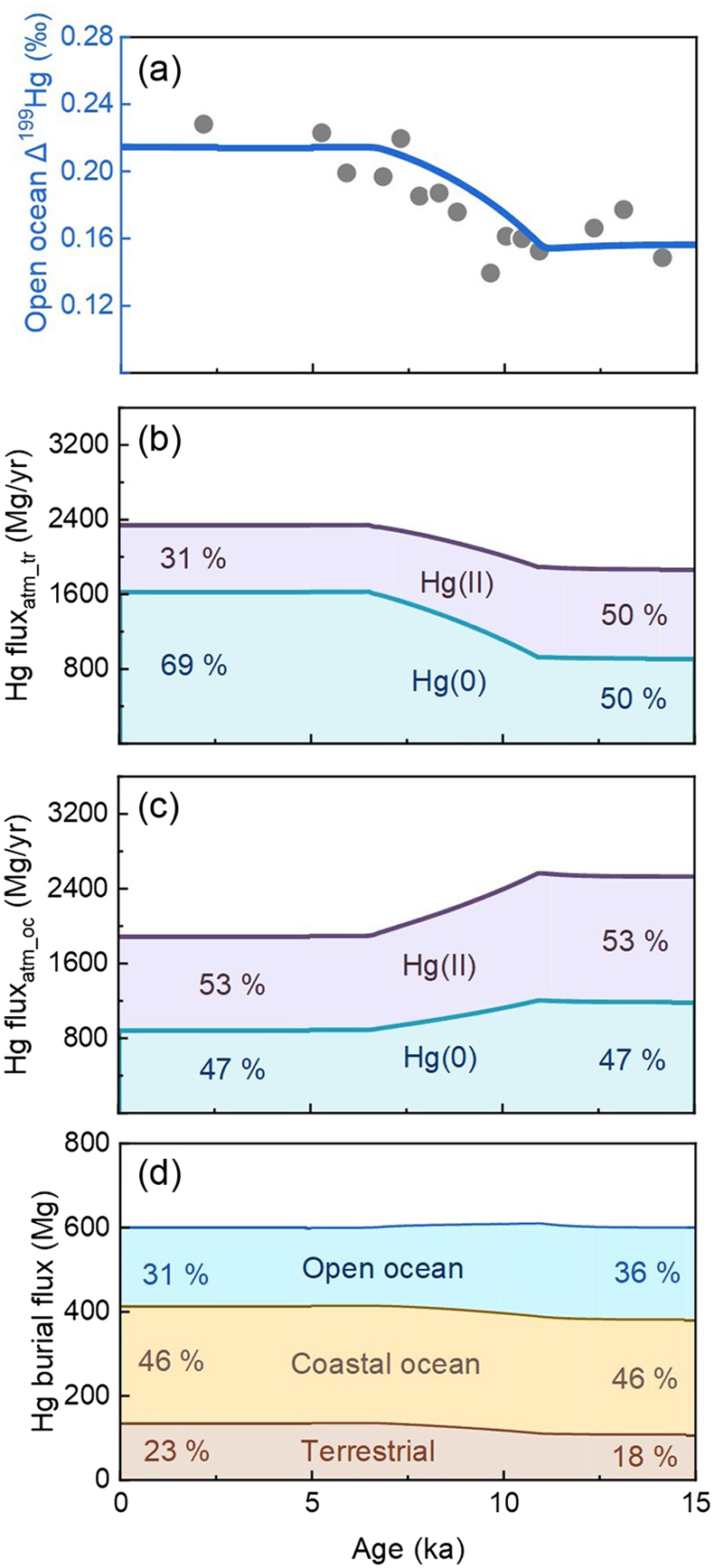
Figure 3 Modelling output illustrating the impact of enhanced atmospheric Hg(0) uptake by the terrestrial system during the early Holocene. (a) The observed (grey points) and model output (blue lines) of the open ocean Δ199Hg. (b) The atmospheric Hg deposition flux to the terrestrial system, with the blue and purple shades indicating Hg(0) and Hg(II) deposition flux, respectively. The percentages indicate the relative contribution of Hg(0) and Hg(II). (c) The atmospheric Hg deposition flux to the open ocean. The shades and percentages are the same as the second row. (d) The Hg burial flux and burial ratio through terrestrial (brown), coastal (yellow), and open ocean (blue) systems.